06 - Multi-Layer Perceptron-Networks

Class: CSCE-421

Notes:

"Now we are talking about something that is not linear"

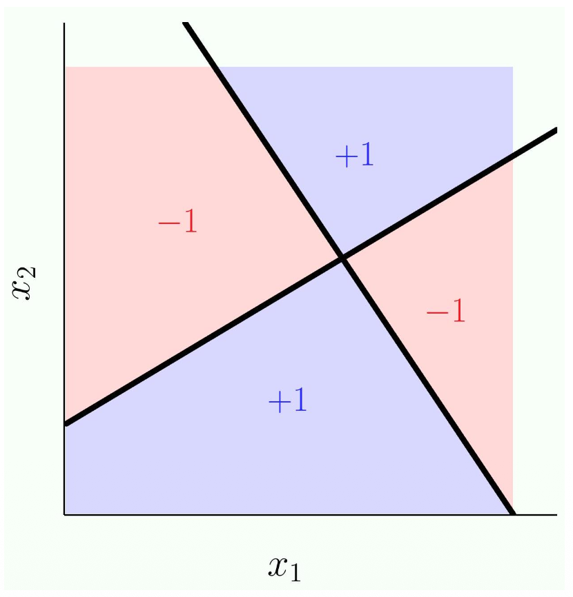
XOR: A Limitation of the Linear Model

The Math

• Linear model: just 2 layers: input layer and output layer
• One way to make this model not linear is to make it wider (still 2 layers)
• This is called kernel methods
  • How to make it wider? you make the input vector to be larger?
  • Usually we do not count the softmax layer
  • The way to make it wider is to apply $\varphi (x)$
    • Now $x$ is a wider vector
    • This model will be not linear in terms of $x$
  • How do we do transformations to a vector $x$?
    • We apply $\varphi$ transformations
    • $\varphi$ is a vector that makes the $x$ components be multiplied by some other $x$ components.
    • You end up increasing the dimension of $x$
• In training, you only need this: $$\phi^T(x_i)\phi(x_j) = (x_i^Tx_j)$$
  • The pairwise inner product with $\varphi$
• There is a more efficient way to do this, which is deep learning (making a model to be deep)
• Kernel methods = use pairwise inner product
  • Can be computed very efficient

The Meaning

1. The Problem: The XOR Limitation Up until now, you have been using simple 2-layer linear models (an input layer $x$ directly connected to an output layer). These models act by drawing a single straight line (or flat plane) to separate the $+1$ class from the $-1$ class.

However, imagine the Exclusive OR (XOR) problem. In a 2D graph, suppose the top-left and bottom-right corners are $+1$, but the top-right and bottom-left corners are $-1$. Try drawing a single straight line to separate the positives from the negatives. You can't. A single linear model is mathematically incapable of solving XOR.

To solve non-linear problems like XOR, we have two main choices: make the model "wider" or make it "deeper".

2. Solution 1: Making it "Wider" (Feature Transforms & Kernel Methods) We already explored making models "wider" in the previous chapter on Polynomial Curve Fitting.

• Feature Transform ($\varphi$): Instead of using the raw input $x$, we apply a mathematical transformation $\varphi (x)$ to stretch $x$ into a much larger, higher-dimensional vector (e.g., by multiplying $x_1$ and $x_2$ together to create new features). Because the input vector is now physically wider, a linear model has more dimensions to work with and can easily draw a flat plane through the wavy data.
• The Kernel Trick: Making vectors infinitely wider takes up massive amounts of computer memory. Your notes mention a shortcut: Kernel Methods. In training algorithms like Support Vector Machines, the algorithm only ever needs to multiply vectors together using a dot product. Instead of computing a giant $\varphi (x_i)$ and a giant $\varphi (x_j)$ and multiplying them, mathematicians discovered formulas that calculate their exact inner product directly from the original tiny $x$ vectors. This is called the "pairwise inner product," and it allows computers to efficiently solve non-linear problems without actually building the giant "wide" vectors.

3. Solution 2: Making it "Deeper" (Deep Learning) Instead of relying on complex math tricks to expand $x$, we can solve the problem by combining multiple simple linear models together. This is the foundation of Deep Learning.

Decomposing XOR

The Math

• Exclusive OR: $f=h_1\overline{h_2}+\overline{h_1}{h}_2$
• Basically means:
  • If $h_1$ and $h_2$ both give you positive or negative, the result is negative (-1).
  • They need to be different for XOR to output positive (+1)
• So they key here is that we use linear models but we use multiple of them and we put them together

The Meaning

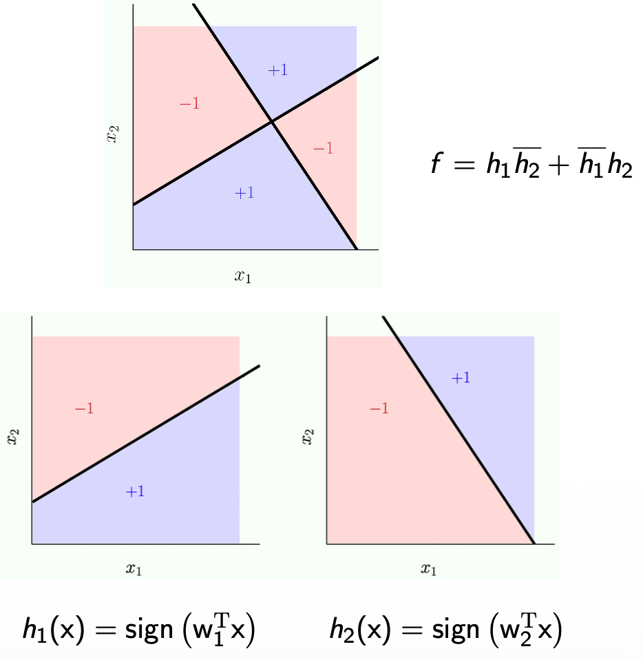
Decomposing XOR These notes prove how multiple linear models can solve XOR using the logic formula: $f=h_1\overline{h_2}+\overline{h_1}{h}_2$. Here is the plain-English breakdown of what this means:

• $h_1$ and $h_2$ are just two entirely separate, standard linear models (two different straight lines drawn on the data).
• The overline (like $\overline{h_2}$) just means "NOT" (or the opposite/negative outcome).
• The formula dictates that the overall final output $f$ will only be positive ($+1$) if $h_1$ and $h_2$ output different answers.
• If both $h_1$ and $h_2$ give a positive answer, or if both give a negative answer, the final outcome is negative ($-1$).

By training two simple linear lines ($h_1$ and $h_2$) and feeding their answers into a new final layer that checks if they match, you have successfully built a multi-layer model that easily solves XOR.

Perceptrons for OR and AND

The Math

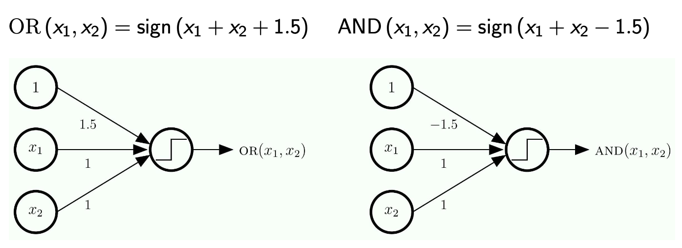
• OR:
  • If one or both of $x_1$ and $x_2$ is positive, then OR is positive
  • Why +1.5?
    • It is just needed to represent OR
    • It will just represent the truth table.
    • The input for $x_1$ and $x_2$ is just +1 or -1
• AND:
  • If both $x_1$ and $x_2$ are positive, then AND is positive

The Meaning

Logic Gates as Simple Perceptrons In the previous slide, we learned that a single linear model cannot solve the XOR problem. However, a single linear model can easily solve basic logic gates like OR and AND. Let's look at how the math works when our inputs ($x_1,x_2$) are strictly $+1$ (True) or $-1$ (False). The slide uses a clever trick with the bias (threshold) weight to switch between OR and AND:

• The OR Perceptron: $\mathrm{sign}(x_1+x_2+1.5)$
  • If both are False ($-1,-1$): $-1-1+1.5=-0.5$. The sign is $-1$ (False).
  • If one is True ($-1,+1$): $-1+1+1.5=+1.5$. The sign is $+1$ (True).
  • If both are True ($+1,+1$): $1+1+1.5=+3.5$. The sign is $+1$ (True).
  • Result: It perfectly mimics an OR gate!
• The AND Perceptron: $\mathrm{sign}(x_1+x_2-1.5)$
  • If one is True ($-1,+1$): $-1+1-1.5=-1.5$. The sign is $-1$ (False).
  • If both are True ($+1,+1$): $1+1-1.5=+0.5$. The sign is $+1$ (True).
  • Result: It only outputs True if both are True, perfectly mimicking an AND gate.

Representing $f$ Using OR and AND

The Math

• Here we work backward because we are given $f=h_1\overline{h_2}+\overline{h_1}{h}_2$
• We need to expand each of $h_1{h}_2$
• Here, $h_1{h}_2$ is the input and the output is $f$

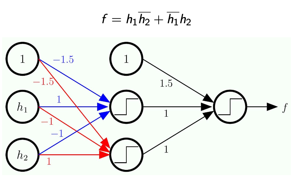
• The next step is to expand each of $h$
  • Note that each of $h_i$ is a linear model of the input
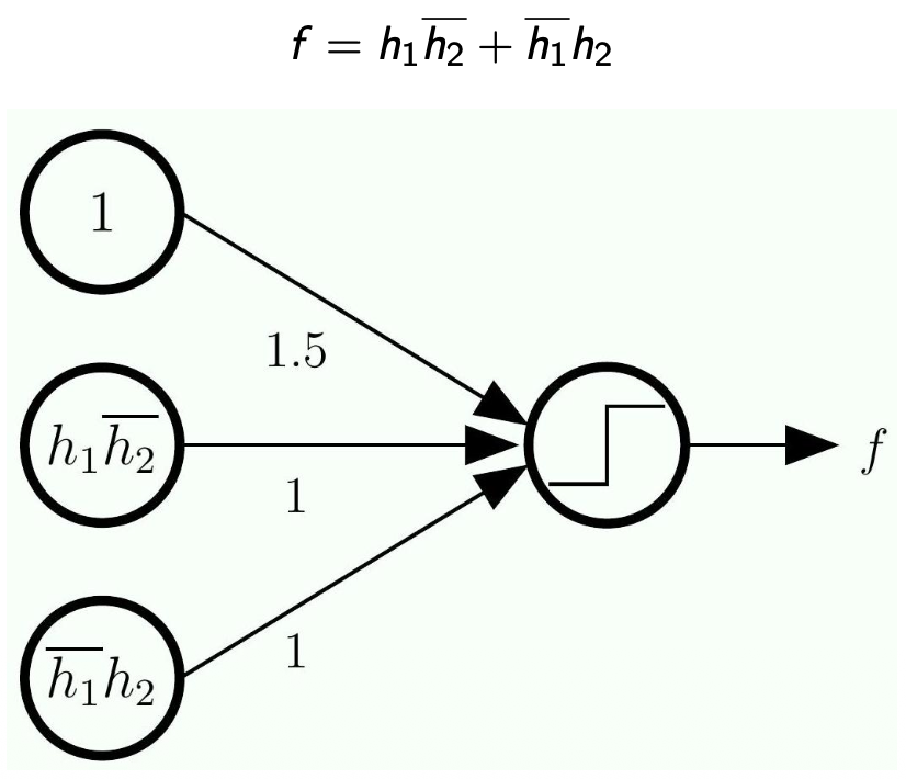
• The -1.5 will eliminate the term we added to implement OR/AND
• Note the bar on the top means $-1$

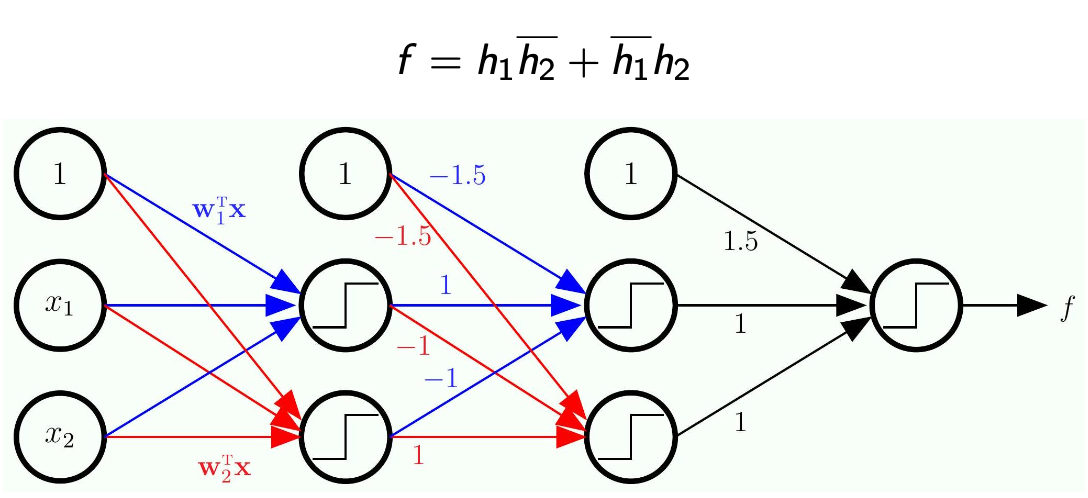
• Now, since we know each of $h_i$ is a linear model of the inputs $x_1$ and $x_2$, then we decompose even more

• Note how this became a network with multiple layers!

• Nothing is trained here

  • This is just a completely hardwire network
  • Solves problems that linear models cannot solve by their own

• Will this method enable us to do more complex models? (something more complex than $f=h_1\overline{h_2}+\overline{h_1}{h}_2$)

  • Yes! you can always convert any logic function into this form
  • As long as you can convert to this standard form you will be used to use a network just like this
    • The logic form will just look longer

The Meaning

1. Representing $f$ (XOR) by Stacking Perceptrons To solve the XOR problem ($f=h_1\overline{h_2}+\overline{h_1}{h}_2$), we cannot use just one perceptron. But, because XOR is just a combination of ANDs, ORs, and NOTs, we can wire multiple perceptrons together.

• Step 1: We calculate our two base linear boundaries ($h_1$ and $h_2$) from the original inputs $x_1$ and $x_2$.
• Step 2: We pass those predictions into a new set of perceptrons acting as AND/OR gates.
• Step 3: The $+1.5$ and $-1.5$ you see inside the circles in your diagram are simply the bias weights ($w_0$) for those specific neurons, perfectly calibrated to execute the OR and AND logic we proved above. The minus signs on the connections act as the "NOT" ($\bar{h}$) operation.

2. Hardwiring vs. Learning Your notes highlight a very important point: "Nothing is trained here. This is just a completely hardwire network". At this stage, we have manually calculated exactly what the weights and biases must be (like the $1.5$ and $-1.5$) to solve XOR. We act as the "designer". In reality, when we build Neural Networks, we don't know what logic gates we need. We just set up the blank architecture (the nodes and connections) and let the Gradient Descent algorithm figure out all the weights and biases on its own! This manual example simply exists to prove mathematically that a multi-layer model is capable of solving a non-linear problem.

The Multilayer Perceptron (MLP)

The Math

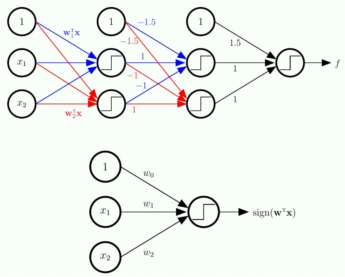
• More layers allow us to implement $f$
• These additional layers are called hidden layers

The Meaning

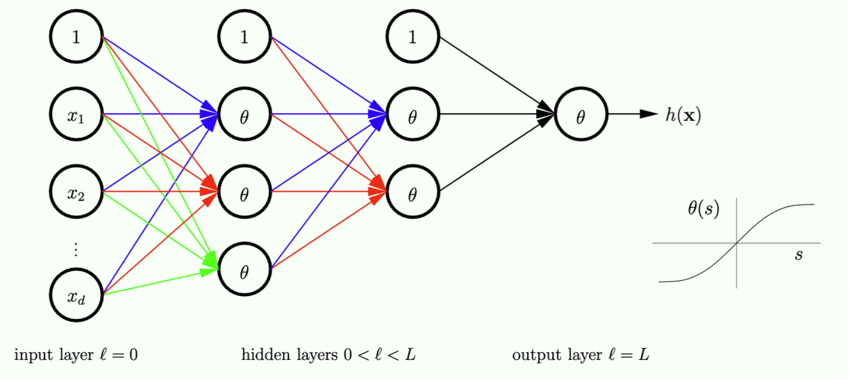
The Multilayer Perceptron (MLP) and Universal Approximation: By feeding the output of one linear model into the input of another, you have created a Multilayer Perceptron (MLP).

• Hidden Layers: The original data is the Input Layer. The final prediction is the Output Layer. Every layer of neurons we sandwich in the middle is called a Hidden Layer.
• Why does this matter? You asked in your notes: "Will this method enable us to do more complex models?" The answer is a resounding Yes. This brings up a famous concept called Universal Approximation.

Universal Approximation

• Any target function $f$ that can be decomposed into linear separators can be implemented by a 3-layer MLP.
• A sufficiently smooth separator can "essentially" be decomposed into linear separators.

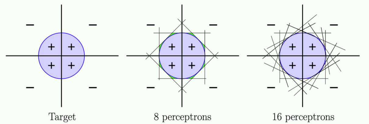
Theory:

• More units/More linear models -> more accurate predictions
• Because you can convert any complex logic function into a combination of basic AND/OR gates, you can technically approximate any target function in the universe just by adding more units and more hidden layers.

The Neural Network

The Math

• $E_{\text{in }}$ is not smooth (due to sign function), so cannot use gradient descent.
• $\mathrm{sign}(x)\approx \tanh (x)⟶$ gradient descent to minimize $E_{\mathrm{in}}$.

• $\theta$ needs to be differentiable
• This function has been used for many years, until recently we changed this, but we will talk about this later
• Note: we use training data to determine all the weights here.
• The question is how do we obtain those connection weights?
  • If I have this values on the left, how do we compute the values on the right (on the next layer)
• The "1" on each layer is essentially the threshold term
  • That is why this unit will have no input, but will have an output of a fixed value
• Note this is not necessarily the most economical way
  • If you use more layers, the total number of units might be smaller, that is why people usually do many many layers, even thousands

The Meaning

1. Why $\tanh (x)$?

• The standard $\mathrm{sign}(x)$ function outputs a hard $-1$ or $+1$. It is a flat line with a sudden, sharp cliff at zero. Because it is flat everywhere else, its gradient (slope) is $0$, making Gradient Descent impossible.
• The Solution: The $\tanh (x)$ function is an S-shaped curve (a "soft threshold") that smoothly transitions from $-1$ to $+1$. Because it is perfectly smooth and has no sharp cliffs, it is everywhere differentiable. This allows the computer to calculate a gradient and use Gradient Descent to learn the weights automatically, rather than us having to hardwire them manually!

2. The Bias Units (The "1" Nodes) Your notes ask about the "1" on each layer. This is the exact same concept as the dummy coordinate $x_0=1$ we used in Linear Regression and the Perceptron.

• Every hidden layer needs its own threshold (bias) to shift the activation function left or right.
• Instead of writing a separate bias term $+b$ for every single node, we just add a "fake" node to every layer that always outputs the number $1$.
• This node has no inputs (no arrows point into it) because its value never changes. It just outputs $1$ and sends it forward to the next layer to be multiplied by the bias weights.

Zooming into a Hidden Node

The Math

layer $\ell$ parameters (notations)

layers $\ell =0,1,2,\dots ,L$
layer $\ell$ has "dimension" ${\mathit{d}}^{(\ell )}⟹{\mathit{d}}^{(\ell )}+1$ nodes

Notes:

• What are the operations to move between layers?
• For each layer we have a signal ($s$) go into a particular layer
• For each layer we want to put the inputs for each unit into a vector, this vector is called ${\mathbf{s}}^{(\ell )}$
  • Note that ${\mathit{d}}^{(\ell )}$ does not consider the bias term
• Summary: each layer has an input vector, and an output vector
• At the end we will build a matrix where each row is one column (one layer)
• What would be the size of this matrix?
  • ${\mathit{d}}^{(\ell -1)}+1\times {\mathit{d}}^{(\ell )}$
    • This will be on the exam!

The Meaning

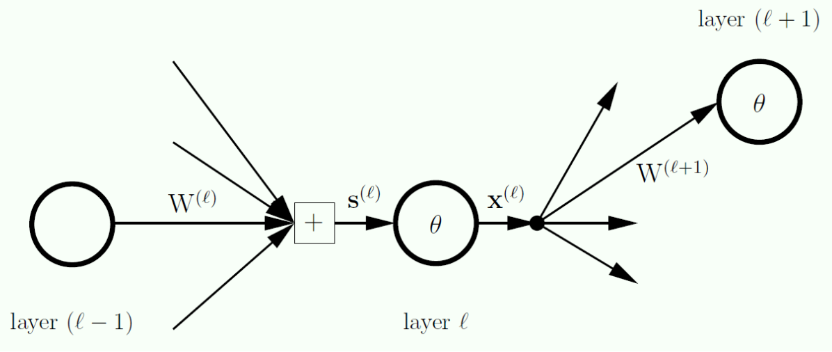
1. Zooming into a Node (The Pipeline) To understand Neural Network math, you must understand the two-step pipeline that happens at every single layer $\ell$.

• Step 1 (The Signal ${\mathbf{s}}^{(\ell )}$): The layer receives raw signals from the previous layer. It multiplies the previous outputs by the weights and adds them up. This results in the $d^{(\ell )}$ dimensional input vector ${\mathbf{s}}^{(\ell )}$.
• Step 2 (The Output ${\mathbf{x}}^{(\ell )}$): The layer passes those raw signals through the smooth activation function ($\tanh$ or $\theta$) to get the final outputs. We then instantly glue a $1$ to the top of this vector for the bias. This makes the output vector ${\mathbf{x}}^{(\ell )}$ slightly larger, with $d^{(\ell )}+1$ dimensions.

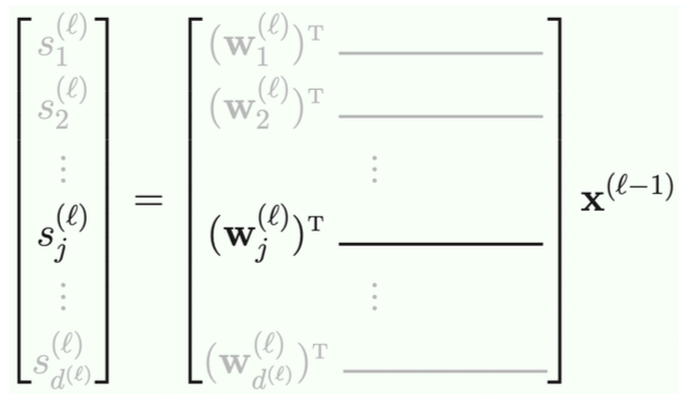
2. Cracking the Exam Question: The Weight Matrix Dimensions Your notes emphasize that the size of the weight matrix $W^{(\ell )}$ will be on the exam. Let's break down why it has the dimensions $({\mathit{d}}^{(\ell -1)}+1)\times {\mathit{d}}^{(\ell )}$ so you don't have to just memorize it.

The matrix $W^{(\ell )}$ is the bridge connecting layer $\ell -1$ to layer $\ell$.

• The Rows (Where the data comes from): The matrix needs a row for every single output coming from the previous layer $\ell -1$. How many outputs did the previous layer have? It had $d^{(\ell -1)}$ regular nodes, PLUS $1$ bias node. Therefore, the matrix needs $d^{(\ell -1)}+1$ rows.
• The Columns (Where the data is going): The matrix needs a column for every single node receiving data in the current layer $\ell$. How many nodes receive data? Only the $d^{(\ell )}$ regular nodes (remember, the bias node in layer $\ell$ generates its own "1" and does not accept incoming signals!). Therefore, the matrix needs $d^{(\ell )}$ columns.

The Linear Signal

The Math

Input ${\mathbf{s}}^{(\ell )}$ is a linear combination (using weights) of the outputs of the previous layer ${\mathrm{x}}^{(\ell -1)}$.

The question:

• If I have the input for one layer, how do we calculate the output?
  • What is the operation? This is $\theta$
    • We need to take a vector and apply $\theta$ to every element (element-wise product with $\theta$)
• Now, If I know the output values for this layer, how do we calculate the input values for the next layer?
  • If you look at the graph, the input of every unit depends on the outputs of the previous layers, but how do we do this?
  • What else do we need? -> the weights
    • We need to take 1 column from the weights matrix.
    • Remember the rows of the weights matrix is composed of the previous layer number of of units as rows and the next layer number of units as columns
      • For example between the second (1, $\theta$, $\theta$, $\theta$) and third layers (1, $\theta$, $\theta$) in the example above we will have a 4 * 2 matrix
      • In order to multiply the weights times the $x$ vector you need to do $x{W}^T$ to account for the different number of rows and columns on each vector/matrix
• The question here is, given the input of a layer, how do we compute the input for the next layer?
  • The operation is simple, you just apply $\theta$
  • Take that vector, apply $\theta$ element-wise and add a 1 (the threshold)
  • Of course the output, by convention needs to be a column vector
  • This is how you get to the form: $s_j^{(\ell )}={\left(w_j^{(\ell )}\right)}^{\mathrm{T}}{\mathrm{x}}^{(\ell -1)}$
• All of this will be in the exam
  • Will ask for number of parameters and stuff

The Meaning

1. The Two-Step Process of a Neural Network Layer Your notes ask an excellent question: "Given the input of a layer, how do we compute the input for the next layer?" It is crucial to clarify the terminology here. Moving data through a Neural Network happens in a repeating two-step cycle for every layer $\ell$:

• Step A (The Bridge): Multiply the outputs of the previous layer (${\mathbf{x}}^{(\ell -1)}$) by the weights to get the raw input signals for the current layer (${\mathbf{s}}^{(\ell )}$).
• Step B (The Activation): Apply the activation function ($\theta$) to those raw signals to get the final outputs of the current layer (${\mathbf{x}}^{(\ell )}$). These outputs are then passed to the next layer.

2. Step A: Calculating the Raw Signal (${\mathbf{s}}^{(\ell )}$) The mathematical formula for the first step is: ${\mathbf{s}}^{(\ell )}={\left({\mathrm{W}}^{(\ell )}\right)}^{\mathrm{T}}{\mathbf{x}}^{(\ell -1)}$.

• Let's look at your example with the $4\times 2$ matrix. You mapped this out perfectly! If layer $\ell -1$ has 3 active nodes + 1 bias node (total 4 outputs), and layer $\ell$ has 2 active nodes, the weight matrix ${\mathrm{W}}^{(\ell )}$ connecting them will have dimensions $4\times 2$.
• To get the input signal for just one specific node $j$ in the new layer, you take the dot product of the $j$-th column of the weight matrix ($w_j^{(\ell )}$) and the output vector from the previous layer.
• Correction to your linear algebra note: You wrote that you need to do "$x{W}^T$". By mathematical convention, because $\mathbf{x}$ is a column vector, you actually evaluate it exactly as written in the slide: $({\mathrm{W}}^{(\ell )}{)}^T{\mathbf{x}}^{(\ell -1)}$. Transposing the $4\times 2$ weight matrix into a $2\times 4$ matrix, and multiplying it by the $4\times 1$ column vector (${\mathbf{x}}^{(\ell -1)}$), results in a neat $2\times 1$ column vector. This is your raw signal vector ${\mathbf{s}}^{(\ell )}$.

3. Step B: Calculating the Output (${\mathbf{x}}^{(\ell )}$) Your notes state: "The operation is simple, you just apply $\theta$. Take that vector, apply $\theta$ element-wise and add a 1." This is absolutely correct and forms the second half of the pipeline.

• You take your raw signal vector ${\mathbf{s}}^{(\ell )}$ and apply the nonlinear $\theta$ function (like $\tanh$) to every single number inside it.
• Then, you must append the number 1 to the very top of the vector. This 1 becomes the dummy bias coordinate for the next layer's calculations.

4. Exam Prep: Counting Parameters You noted that the exam will ask for the number of parameters. In a neural network, the "parameters" are simply the total number of weights (the individual elements inside the $\mathrm{W}$ matrices).

• For a single layer transition, the number of parameters is exactly the number of rows multiplied by the number of columns in ${\mathrm{W}}^{(\ell )}$.
• Formula: $(d^{(\ell -1)}+1)\times d^{(\ell )}$.
• Example: For your $4\times 2$ matrix transition, there are exactly $4\times 2=8$ parameters (weights) to learn for that specific layer.

Forward Propagation: Computing $h(x)$

Forward propagation to compute $h(\mathrm{x})$:

1. ${\mathrm{X}}^{(0)}\leftarrow \mathrm{X}$
   • [Initialization]
2. for $\ell =1$ to $L$ do
   • [Forward Propagation]
3. ${\mathrm{s}}^{(\ell )}\leftarrow {\left({\mathrm{W}}^{(\ell )}\right)}^{\mathrm{T}}{\mathrm{x}}^{(\ell -1)}$
4. ${\mathrm{x}}^{(\ell )}\leftarrow \left[\begin{array}{c}1\\ \theta \left({\mathrm{s}}^{(\ell )}\right)\end{array}\right]$
5. end for
6. $h(\mathrm{x})={\mathrm{x}}^{(L)}$
   • [Output]

Notes:

• You have x, where you want to make preditions
• Input layer is x(0), (there is no $\theta$ in the input layer)
• To compute the input to the next layer we apply $w(1)$, then to get to the next layer you apply $\theta$, and so on, you repeat this process.
• There are 2 operations to reach a next layer

Minimizing Ein

The Math

Using $\theta =\tanh$ makes $E_{\text{in }}$ differentiable so we can use gradient descent ⟶ local minimum.

Notes:

• Now this is about prediction.
• A backward propagation is to adjust weights after a training process and then you need to do forward propagation
• The cost of training the network using a simple example is twice the price of doing a prediction
• Given some samples, how do you train your network?
• We will write a loop and iteratively update each of the $w$ weights.

The Meaning

1. The Objective: Minimizing the Error ($E_{in}$) Just like in linear regression, the goal of training a neural network is to find the weights that make our predictions ($h(x_n)$) as close to the true labels ($y_n$) as possible. The slide uses the standard squared error function: $$E_{\text {in }}(\mathrm{W})=\frac{1}{N} \sum_{n=1}^N\left(h\left(\mathrm{x}_n\right)-y_n\right)^2$$

• Why $\tanh$? The slide reminds us that we must use a smooth activation function like $\tanh$ (or the logistic sigmoid $\theta$) instead of a hard sign() threshold. If we used a hard step function, the error landscape would be a flat plateau with sudden cliffs. The gradient (slope) would be exactly zero almost everywhere, meaning the computer wouldn't know which way to step. Because $\tanh$ is smooth, $E_{in}$ becomes differentiable, allowing us to roll down the hill to a local minimum.

2. Correcting your note: The Training Cycle In your notes, you wrote: "A backward propagation is to adjust weights after a training process and then you need to do forward propagation." It is important to get the order of operations exactly right for your exam. One single step of training actually happens in this exact order:

1. Forward Propagation: Pass a data point $x$ through the network to get a prediction $h(x)$, and calculate how wrong it is (the error).
2. Backward Propagation (Backprop): Use the Chain Rule to calculate the gradient (the slope) of that error with respect to every single weight in the network.
3. Weight Update (Gradient Descent): Adjust the weights by taking a small step in the negative gradient direction.

• Note on Computational Cost: You correctly noted that training is about twice as expensive as predicting. Making a prediction requires one pass (Forward). Training requires both a Forward pass (to get the values) and a Backward pass (to compute the derivatives/slopes).

Gradient Descent

The Math

Notes:

• Think about the $W$ to be the collection of all $w$ weights.
• The key here is still how to compute the derivative, then you plug in $W(t)$ and move in a negative direction.
• $\eta$ is pretty much empirical, and is pretty much this way for all training models, but the hard part is the gradient part.

The Meaning

The Gradient Descent Update Rule Because a neural network has multiple layers, the "weight" parameter $\mathrm{W}$ is no longer just one vector. It is a massive collection of several matrices $\{{\mathrm{W}}^{(1)},{\mathrm{W}}^{(2)},\dots ,{\mathrm{W}}^{(L)}\}$, one for each layer. To update all these matrices at once, we use the standard Gradient Descent rule: $$\mathrm{W}(t+1)=\mathrm{W}(t)-\eta \nabla E_{\mathrm{in}}(\mathrm{~W}(t))$$

• $\eta$ (Learning Rate): As you noted, this is chosen empirically (often through trial and error or validation). It determines how big of a step we take.
• $\mathrm{\nabla }{E}_{in}$ (The Gradient): This is the massive matrix of slopes for every single weight in the network. Finding this is the hardest part of Deep Learning.

Gradient of Ein

The Math

We need

Notes:

• To compute the gradient, pretty much you need to repeatedly use the chain rule (Computing this derivative is nothing but chain rule)
• Instead of going through all the details we will just review the results intuitively.
• Again, you need to know if we have a loss function Ein, you compute the loss function of every sample and then you do a summation of all of those
  • If you can get the loss for a single sample, then you can just do summation of all the samples to get the total loss
  • We just need to get the gradient of a single sample and then just do a summation.

The Meaning

Divide and Conquer: The Gradient of One Sample How do we calculate the derivative for a massive network over a dataset of thousands of images? The slide shows a brilliant mathematical shortcut: Divide and Conquer.

The total error $E_{in}$ is just the average of the individual errors ($e_n$) for every single data point. Because the derivative of a sum is just the sum of the derivatives, we can pull the derivative operator inside the summation: $$\frac{\partial E_{\mathrm{in}}(\mathrm{w})}{\partial \mathrm{W}^{(\ell)}} = \frac{1}{N} \sum_{n=1}^N \frac{\partial \mathrm{e}_n}{\partial \mathrm{~W}^{(\ell)}}$$What does this mean in plain English? It means we do not need to figure out the calculus for the entire dataset at once. We only need to figure out how to calculate the gradient for one single data point ($\frac{\partial \mathrm{e}}{\partial {\mathrm{W}}^{(\ell )}}$). Once we use the Chain Rule to find the derivative for one point, we simply run a loop: calculate the derivative for point 1, point 2, point 3... and then average them all together to get the true gradient for the whole dataset.

Algorithmic Approach

The Math

$\mathrm{e}(\mathrm{x})$ is a function of ${\mathrm{s}}^{(\ell )}$ and ${\mathrm{s}}^{(\ell )}={\left({\mathrm{W}}^{(\ell )}\right)}^{\mathrm{T}}{\mathrm{x}}^{(\ell -1)}$

sensitivity

Notes:

• We need to derive one more thing, called sensitivity.
  • Above is the definition of sensitivity
  • It is a vector, and there is a sensitivity for each layer
  • It is the partial derivate of the error (just a number) in terms of the partial derivative of each element of $s^{(\ell )}$ (the input vector into this layer)
• But what does sensitivity measure?
  • Look at it element-wise
  • Basically it measures how much the input affects the error (e)
  • This is essentially the idea of a partial derivative, if you have a unit change of the input, how much the output would change?
    • Think of getting the derivative of y = 2x in terms of y?
    • It is just 2, this means if the input is increased by one unit, the output is increased by two units.
  • If we have unit change in the input, how much will it change on e?
  • If the sensitivity for a unit is 0, it will not affect e

Notes:

• $W$ is the connection between two layers
• So now we want to know the partial derivative of the error in terms of $W$
• Remember rows come from the previous layer (i), and columns come from the next layer (j)
• What we want to answer is: If this $W$ is changed by a small amount, how much will $e$ change?
  • If we have unit change in each of the $W$, how much it changes the error?
• What do we need to know to compute this?
  • Suppose you know the sensitivity of every layer
  • What affects the derivative of $W$?
  • If the sensitivity for a unit is large, that means if we have a small change in one entry, the change in error is large, you do not need to consider anything downstream,
    • The sensitivity basically tells you everything after this layer encoded into a single vector
  • What else is important here?
    • If the output unit if (i) has a zero value, and the derivative measure if we have unit change with the connection $W$, what would happen here?
    • This output value is multiplied with $W$, then what would happen to j? There is no change, the derivative is 0.
• The derivative of $W$ is simply the output value of (i) times the sensitivity value of (j)
• If you connect all of that into a matrix you get to: ${\mathrm{x}}^{(\ell -1)}{\left({\mathit{\delta }}^{(\ell )}\right)}^{\mathrm{T}}$
  • How can we obtain $x$?
    • Again we are talking about a single sample, because if we can do this for a single sample, we can do this for every sample
    • Just use the #Forward Propagation Computing $h(x)$ formula, if you do forward propagation you get the $x$ for each layer.
• Question: $W$s are randomly initialized, what happens if we initialize $W$ to be all zeroes? what will happen?
  • In logistic regression you can do that because you only have one layer, but what would be the consequence here?
  • This is an exam question, if you have a network of layers, is initializing $W$ to be all zeroes a good idea?
  • It is not a good idea because if we do it (a zero matrix) in forward propagation, the values on the output will be all zero vectors, and with $\theta$, if the input is zero, the output will be zero, so the $x$ of the next layer will be all zeros.
• Takeaway: the derivate in terms of W is proportional to the sensitivity.

The Meaning

1. The Goal: Finding the Gradient To train the neural network, we need to know how to adjust every single weight matrix $W^{(\ell )}$ to make the final error $e$ smaller. Mathematically, we need to find $\frac{\partial \mathrm{e}}{\partial {\mathrm{W}}^{(\ell )}}$. However, the weights $W^{(\ell )}$ do not directly calculate the error. The weights calculate the raw signal $s^{(\ell )}$, which goes through an activation function to become $x^{(\ell )}$, which eventually goes to the output layer to calculate the error. Because of this chain of events, we must use the Chain Rule from calculus.

2. The Chain Rule Split The slide splits the impossible derivative into two manageable pieces multiplied together: $$ \frac{\partial \mathrm{e}}{\partial \mathrm{W}^{(\ell)}} = \frac{\partial \mathrm{s}^{(\ell)}}{\partial \mathrm{W}^{(\ell)}} \cdot \left(\frac{\partial \mathrm{e}}{\partial \mathrm{s}^{(\ell)}}\right)^T $$

• Part 1: $\frac{\partial {\mathrm{s}}^{(\ell )}}{\partial {\mathrm{W}}^{(\ell )}}$: How much do the weights change the raw signal? Because the raw signal is just $s=W^{T}x$, the derivative with respect to $W$ is simply the input data $x^{(\ell -1)}$ from the previous layer.
• Part 2: $\frac{\partial \mathrm{e}}{\partial {\mathrm{s}}^{(\ell )}}$: How much does the raw signal change the final error? We define this specific piece as a brand new variable: Sensitivity (${\delta }^{(\ell )}$).

3. What is Sensitivity ($\delta$)? Your notes on this are excellent! You correctly point out that sensitivity measures exactly how much a change in the raw input signal affects the final error $e$.

• Because $s^{(\ell )}$ is a vector (one raw signal for every node in layer $\ell$), the sensitivity ${\delta }^{(\ell )}$ is also a vector. It contains a separate derivative for every single node in that layer.
• Your $y=2x$ analogy is spot on. If the sensitivity $\delta$ for a specific node is $2$, it means that if we nudge that node's raw signal up by $1$ unit, the total network error will increase by $2$ units.
• If the sensitivity is $0$, the network's error is completely "numb" to that node. You could change that node's signal, and the final error wouldn't budge at all.
• Note: The $\delta$ vector acts as a summary. It encodes everything that happens downstream in the network into a single convenient number for each node.

4. Putting it Together (The Matrix Math) When we substitute $x^{(\ell -1)}$ and ${\delta }^{(\ell )}$ back into the Chain Rule equation, we get the final brilliant formula for the gradient: $$ \frac{\partial \mathrm{e}}{\partial \mathrm{W}^{(\ell)}} = \mathrm{x}^{(\ell-1)}\left(\boldsymbol{\delta}^{(\ell)}\right)^{\mathrm{T}} $$ Let's look at why this makes perfect sense, both logically and mathematically:

• The Logic: To figure out how much to tweak the weight connecting Node A to Node B, you only need to know two things: How strong was the signal coming out of Node A ($x$), and how sensitive is the error to what goes into Node B ($\delta$).
• The Math (Exam Tip!): Remember in your previous notes you learned the dimensions of the weight matrix $W^{(\ell )}$ are $(d^{(\ell -1)}+1)\times d^{(\ell )}$? Look at the vector multiplication here. You are multiplying a column vector $x^{(\ell -1)}$ (which has $d^{(\ell -1)}+1$ rows) by a transposed row vector $({\delta }^{(\ell )}{)}^T$ (which has $d^{(\ell )}$ columns). In linear algebra, multiplying a column by a row is called an Outer Product, and it perfectly creates a matrix of size $(d^{(\ell -1)}+1)\times d^{(\ell )}$! Every single weight gets its own unique slope calculated instantly.

5. The Formula: Slope = Input $\times$ Sensitivity You are looking at the final formula from the Chain Rule: $\frac{\partial \mathrm{e}}{\partial W^{(\ell )}}={\mathrm{x}}^{(\ell -1)}{\left({\mathit{\delta }}^{(\ell )}\right)}^{\mathrm{T}}$. Let's translate this matrix math into plain English for a single weight connecting Node $i$ to Node $j$:

• The Question: "If I tweak this exact weight by 1 unit, how much does my final error change?"
• The Answer: It depends entirely on two things:
  1. $x_i$ (The Signal Strength): How loud is Node $i$ shouting? If Node $i$ is outputting a $0$, it doesn't matter how much you tweak the weight connecting it to Node $j$. Any weight multiplied by $0$ is still $0$. Therefore, if $x_i=0$, tweaking the weight has absolutely no effect on the network, so the derivative (slope) is exactly $0$.
  2. ${\delta }_j$ (The Sensitivity): How much does the final error care about what enters Node $j$? If the downstream network is highly sensitive to Node $j$, then ${\delta }_j$ is large. A small tweak to the weight will cause a massive change in the error.

6. Where do we get these numbers? As your notes point out, you get these two pieces of the puzzle at two different times:

• $x^{(\ell -1)}$ (The Inputs): You get this for free during Forward Propagation. As you pass the image/data through the network to make a prediction, you just save the outputs of every layer in the computer's memory.
• ${\delta }^{(\ell )}$ (The Sensitivities): You calculate these during Backward Propagation (which we will look at in the next slide).

7. CRITICAL EXAM CONCEPT: The "All-Zeros" Initialization Your notes bring up a classic, guaranteed exam question: "What happens if we initialize $W$ to be all zeroes?"

Your notes answer this by saying that if $W=0$, the input to the activation function is $0$. If you are using $\tanh$, then $\tanh (0)=0$, meaning the output $x$ of all your hidden nodes becomes $0$, paralyzing the network. This is completely true! However, there is an even bigger, more fundamental reason why this fails, which professors specifically look for: The Symmetry Breaking Problem.

Imagine you use the Logistic Sigmoid function instead, where $\theta (0)=0.5$. The outputs are no longer zero. Does initializing with all zeros work now? No!

• If every single weight is $0$, then every single node in a hidden layer receives the exact same input signal.
• Because they receive the exact same input, they will output the exact same value.
• During backpropagation, they will all calculate the exact same sensitivity ($\delta$) and the exact same gradient.
• When Gradient Descent updates the weights, it will change every single weight by the exact same amount.

If you have 1,000 hidden nodes, but they all have the exact same weights and do the exact same math, you don't actually have 1,000 nodes—you effectively just have 1 node. The network will never be able to learn different, complex features (like one node looking for edges, and another looking for colors). Therefore, you must initialize weights with small, random numbers to "break the symmetry" so that different nodes can learn different things!

Computing ${\delta }^{(\ell )}$ Using the Chain Rule

The Math

Multiple applications of the chain rule:

Notes:

• To compute the sensitivity we use backward propagation, we start from the last layer, until we reach the first one.
• All we need to do is given a particular delta, how do we compute the delta from the previous layer
• Delta is a derivate, so we need to backward propagate this derivative, so we are propagating derivatives
• Easier case: Given delta (l), how do we calculate delta (l-1)?
  • Basically you need to know the partial derivative to the output
  • If we know the partial derivative of the output for this layer , how do we calculate the partial derivative of the input.
    • Note you are not propagating the actual value, you are propagating the derivative
  • You have to compute the derivative of $\theta$ to get a function, and then you need to plug in to the value you got from forward propagation
• Why this is important?
  • You can see that if you take the derivate of $\theta (s)$ the derivative will be close to 0.
    • If your input value to $\theta$ is very large, your gradient will be close to 0.
• The backward propagation in some units will depend on the forward propagation, that is why we first need to do forward propagation.
• Why is this non-linear function a curve gradient?
  • When we talk about $\theta$ we are talking about element-wise (each unit)
  • You compute the gradient of $\theta$, and the you plug in.
  • If $W$ has a grater gradient in the output, the input will be close to 0.

Notes:

• How do we backward propagate the W matrix
• It requires two operations
  • We need to first forward propagate
  • Then we need forward propagation
• The weight (each line) needs to be multiplied with the sensitivity on each unit, then we'll sum them up together and get the derivative
• You are taking the ith row and taking the inner product with each sensitivity (each column). This is represented as a matrix multiplication
  • This is because this product eventually becomes a column vector
  • Multiply W matrix with the sensitivity vector, but note you are removing the first element.
  • The 1 does not need to be backward propagated because there is no input for the "1" entry.
• Note that during prediction time you just need forward propagation, but in training you will need to do forward propagation first, then you need to do backward propagation
  • The cost of doing forward propagation is twice the cost of doing backward propagation
    • In forward propagation we do matrix multiplication
    • In forward propagation we again multiply this W but elementwise?
  • This is why training a network is much more expensive.

The Meaning

1. The Big Picture: Passing the Blame Backwards In the previous slide, we learned that to update the weights, we need to know the Sensitivity (${\delta }^{(\ell )}$) of every single layer.

• For the very last layer (the output layer $L$), this is easy. We know the exact prediction, we know the true answer, so we can directly calculate the error derivative.
• But how do we find the sensitivity of the hidden layers deep inside the network? We use Backward Propagation. We start with the sensitivity at the output layer (${\delta }^{(L)}$) and use the Chain Rule to pass the "blame" for the error backwards through the network: ${\delta }^{(L)}\to {\delta }^{(L-1)}\to \cdots \to {\delta }^{(1)}$.

2. Breaking Down the Backprop Formula Your slide gives the master formula for how to compute the sensitivity of the current layer ($\ell$) if you already know the sensitivity of the next layer ($\ell +1$): $$ \boldsymbol{\delta}^{(\ell)}=\theta^{\prime}\left(\mathbf{s}^{(\ell)}\right) \otimes\left[\mathrm{W}^{(\ell+1)} \boldsymbol{\delta}^{(\ell+1)}\right]_1^{d^{(\ell)}} $$ This formula executes the two "backward" steps required to pass through a layer:

• Step A: Moving backward across the weights ($W^{(\ell +1)}$). We take the sensitivities of the next layer (${\delta }^{(\ell +1)}$) and multiply them by the weight matrix connecting the two layers. This calculates how much the outputs ($x^{(\ell )}$) of our current layer contributed to the error.
  • The Bias Note: Your notes say "Multiply W matrix... but note you are removing the first element." This is what the subscript ${}_1^{d^{(\ell )}}$ means. When we compute the errors, we must discard the sensitivity for the bias node (the "1"). Why? Because the bias node is a hardcoded constant 1. It has no inputs, nothing feeds into it, so we do not backpropagate error through it.
• Step B: Moving backward through the activation function ($\theta$). Now that we know the error of the output $x^{(\ell )}$, we need the error of the raw signal $s^{(\ell )}$ (which is what ${\delta }^{(\ell )}$ actually is). To go backwards through a function, calculus tells us we must multiply by its derivative: ${\theta }^{\prime }(s^{(\ell )})$.
  • The $\otimes$ symbol just means element-wise multiplication. We match up the nodes one by one and multiply their values together.

3. The "Curve Gradient" and the Vanishing Gradient Problem You wrote a brilliant note here: "If your input value to $\theta$ is very large, your gradient will be close to 0."

Let's think about why this is mathematically true and practically dangerous:

• If you use $\tanh (s)$ or the logistic sigmoid function $\theta (s)$ as your activation function, they look like an "S" curve. The middle of the "S" is steep, but the far left and far right ends flatten out completely into horizontal lines.
• If a raw signal $s$ is very large (say, $+50$ or $-50$), it lands on the flat part of the curve. The slope (derivative ${\theta }^{\prime }$) of a flat horizontal line is exactly $0$.
• Look back at our Backprop formula: it multiplies by ${\theta }^{\prime }(s^{(\ell )})$. If this derivative is $0$, the entire sensitivity ${\delta }^{(\ell )}$ becomes $0$.
• If $\delta =0$, the weights stop updating (remember the previous slide: $\text{Gradient}=x\cdot \delta$). The network becomes paralyzed and completely stops learning. This is a famous phenomenon in deep learning called the Vanishing Gradient Problem.

The Backpropagation Algorithm

Algorithm for Gradient Descent on Ein

• This is the whole training process
• The key is the inner for loop, it will compute the gradient
  • You do not need to implement this loop in HW2, you will just use pytorch function to do this.
• Can do batch version or sequential version (SGD).

Digits Data