05 - A Unified View of Loss Functions in Supervised Learning

Class: CSCE-421

Notes:

Intro

• So far we have only talk about two different loss functions and two different type of models, linear regression, and logistic regression.
• The loss is how you measure the difference between a predicted value and the real target (label)
  • In Linear regression we use least squares
  • In logistic regression we use the cross-entropy loss
• Today we will be dealing with a more general view of loss functions and other considerations

A Unified View of Loss Functions: Binary-Class Classifier

(1) Given a dataset $X=[{\mathrm{x}}_1,{\mathrm{x}}_2,\dots ,{\mathrm{x}}_n]$ with the corresponding label $Y=[y_1,y_2,\dots ,y_n]$, where ${\mathrm{x}}_i\in {\mathbb{R}}^{d+1}$ and $y_i\in \{+1,-1\}$.

• X is our input vector
• y is our labels vector
• Note this is a two-class (binary) predictor

(2) For a given sample ${\mathrm{x}}_i$, a linear classifier computes the linear score $s_i$ as

(3) We study the relations between loss values and $y_i{s}_i$ :

• Predict -1 if $s_i$ is negative
• Predict +1 if $s_i$ is positive
• ⟹ Prediction is correct if $y_i{s}_i>0$
• Prediction confidence is large if $\left|s_i\right|$ is large
• ⟹ Prediction is very correct if $y_i{s}_i\gg 0$
• ⟹ Prediction is very wrong if $y_i{s}_i\ll 0$

Notes:

• Our predictions are based on $s_i$
• If the $s_i$ is positive you predict (+1), otherwise (-1)
• Now after knowing our prediction we can put it the true label with the score. If these two are different, the prediction will be wrong, but if they are equal the prediction will be correct
  • Note both $y_i$ and $s_i$ need to be of the same sign to yield a correct prediction.
• If $s_i$ has a large magnitude, then the prediction confidence is large, you have a high score!
• Similarly,
  • if $y_i{s}_i$ is very positive (much larger than 0) you have a very confident prediction
  • if $y_i{s}_i$ is very negative (much smaller than 0) you have a very wrong prediction

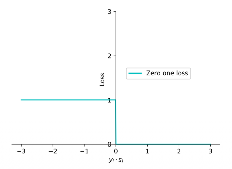
Zero-One Loss

(1) Prediction is correct if $y_i{s}_i>0$

(2) The zero-one loss aims at measuring the number of prediction errors

(3) The loss for the entire training data is $\frac{1}{n}\sum _{i=1}^n{L}_{0/1}(y_i,s_i)$

Notes:

• The first loss function that we will talk about
• It will be 1 when $y_i{s}_i$ is negative and 0 if $y_i{s}_i$ is positive
• What does this loss do?
  • We know that any sample below $y_i{s}_i=0$ is wrong and above that is correct
  • This will just give you a n integer number of how many samples are mis-predicting
• If we want to minimize the training loss
  • If we use the zero-one loss we are just minimizing the number of long predictions
• This loss function is not commonly used because it is not continuous, you will have to deal with discrete optimization (since there is a jump from 0 to 1)
  • The cross-entropy loss is a continuous optimization of this functions

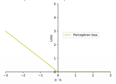
Perceptron loss

(1) The zero-one loss incurs the same loss value of 1 for all wrong predictions, no matter how far a wrong prediction is from the hyperplane.

(2) The perceptron loss addresses this by penalizing each wrong prediction by the extent of violation. The perceptron loss function is defined as $\frac{1}{n}\sum _{i=1}^n{L}_p(y_i,s_i)$, where $L_p$ is perceptron loss which can be described as

(3) Note that the loss is 0 when the input example is correctly classified. The loss is proportional to a quantification of the extent of violation ( $-y_i{s}_i$ ) when the input example is incorrectly classified.

Notes:

• I f$y_i{s}_i$ is positive then you have a positive value as max, if $y_i{s}_i$ is negative then you will have a negative value as max?
• Somehow this loss seems to work right
• It will not give you the number of mis-predictions
• Is an approximation of the zero-one function

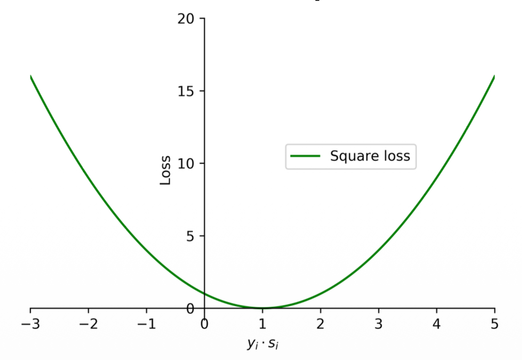
Square loss

(1) The square loss function is commonly used for regression problems.

(2) It can also be used for binary classification problems as

where $L_s$ is the square loss, defined as

(3) Note that the square loss tends to penalize wrong predictions excessively. In addition, when the value of $y_i{s}_i$ is large and the classifier is making correct predictions, the square loss incurs a large loss value.

Notes:

• This will not perform well because whenever you have a correct prediction the loss will still be high!

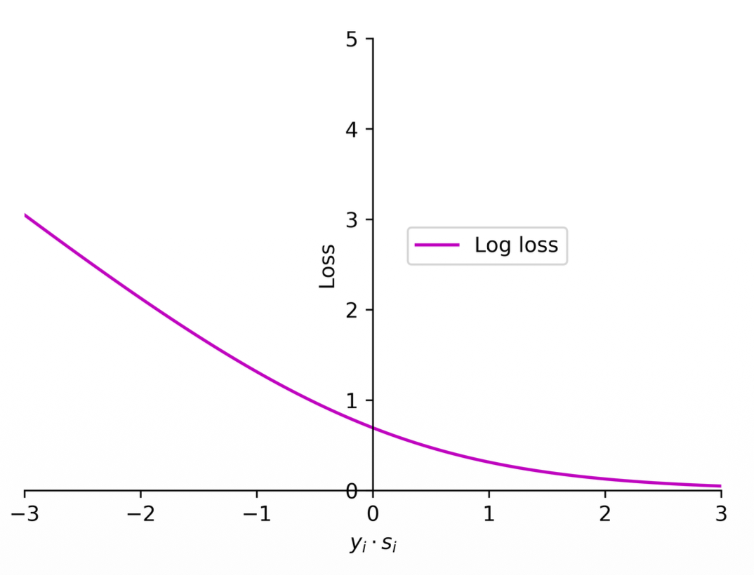
Log loss (cross entropy)

(1) Logistic regression employs the log loss (cross entropy) to train classifiers.

(2) The loss function used in logistic regression can be expressed as

where $L_{\text{log }}$ is the log loss, defined as

Notes:

• Note this is still some kind of approximation of the zero-one loss
• This is commonly used because it is a continuous function and differentiable everywhere
• What is the difference between Perceptron loss and cross entropy loss?
  • Should there be some loss close to 0 or not?
    • Yes, even though it is positive, it is small and represents a weak prediction even though it is correct, we can measure this with the Log loss by applying some loss closer to the 0 boundary
    • The Log loss basically makes it so that the bigger the number (positive) the less the loss.
  • The cross entropy loss is not differentiable (it has a sharp edge)
  • For logistic regression there is no perfect sample, every sample has some loss
    • For strong predictions this value would be very small but never will be zero
    • This is because of how logs work (horizontal asymptote at 0)

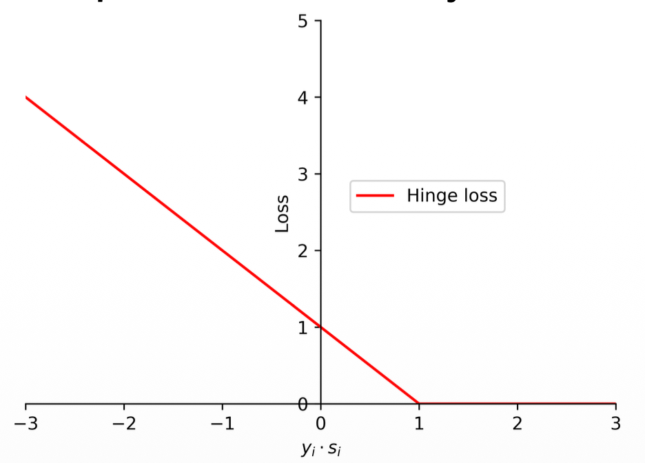
Hinge loss (support vector machines)

(1) The support vector machines employ hinge loss to obtain a classifier with "maximum-margin".

(2) The loss function in support vector machines is defined as follows:

where $L_h$ is the hinge loss:

(3) Different with the zero-one loss and perceptron loss, a data may be penalized even if it is predicted correctly.

Notes:

• Differences of the Hinge loss
  • Note the difference from perceptron loss:
    • Perceptron loss: $max(0,-y_i{s}_i)$
    • Hinge loss: $max(0,1-y_i{s}_i)$
  • The only difference is that 1, and it has a significant impact
    • Essentially it shifts the curve by 1.
    • This applies some loss for the positive predictions closer to 0, like the log loss
    • But still is not a differentiable function
  • Note the log loss would still be a little bit more harsh on positive predictions closer to 0 (applies a bit more loss)
  • The reason we use this is because it could be the case that fits better our data helping the maximum margin (the distance between the loss line and the data points)
    • The reason it is called maximum margin is because of that small loss that applies to weak correct predictions
• Support and non-support vectors:
  • If a data point has zero loss, if you remove this data point, and re-train, the model will remain the same.
    • These are called non-support vectors (points that if removed, the model will remain the same)
    • The other data points are support vectors (incorrect predictions and closer to 0 correct predictions)
    • Look for a visual example of support and non-support vectors
      • To distinguish these two is not trivial, because you need to identify all the data points and how the maximum margin would change if removed
• Something interesting:
  • Why is it 1? Why shifting by 1? is there any difference if we put a 5 there? What would be the difference?
  • If you make it 0 it will just care about if predictions are correct or not (just like perceptron)
  • If you use any positive number the effect will be the same!
    • Regardless of by how many you scale, the margin will remain the same
    • You can use any number! It is just a scale.
  • The only reason that this loss is not really used in deep learning is because it only works for two classes.

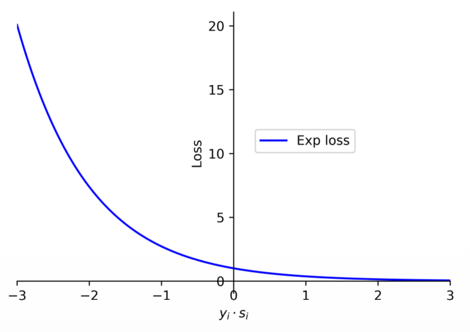
Exponential Loss

(1) The log term in the log loss encourages the loss to grow slowly for negative values, making it less sensitive to wrong predictions.

(2) There is a more aggressive loss function, known as the exponential loss, which grows exponentially for negative values and is thus very sensitive to wrong predictions. The AdaBoost algorithm employs the exponential loss to train the models.

(3) The exponential loss function can be expressed as $\frac{1}{n}\sum _{i=1}^n{L}_{\exp }(y_i,s_i)$, where $L_{\text{exp }}$ is the exponential loss, defined as

Notes:

• Some commercial models and libraries use this loss
• It penalizes data points that are wrong and be a little bit more permissive in correct predictions closer to 0.

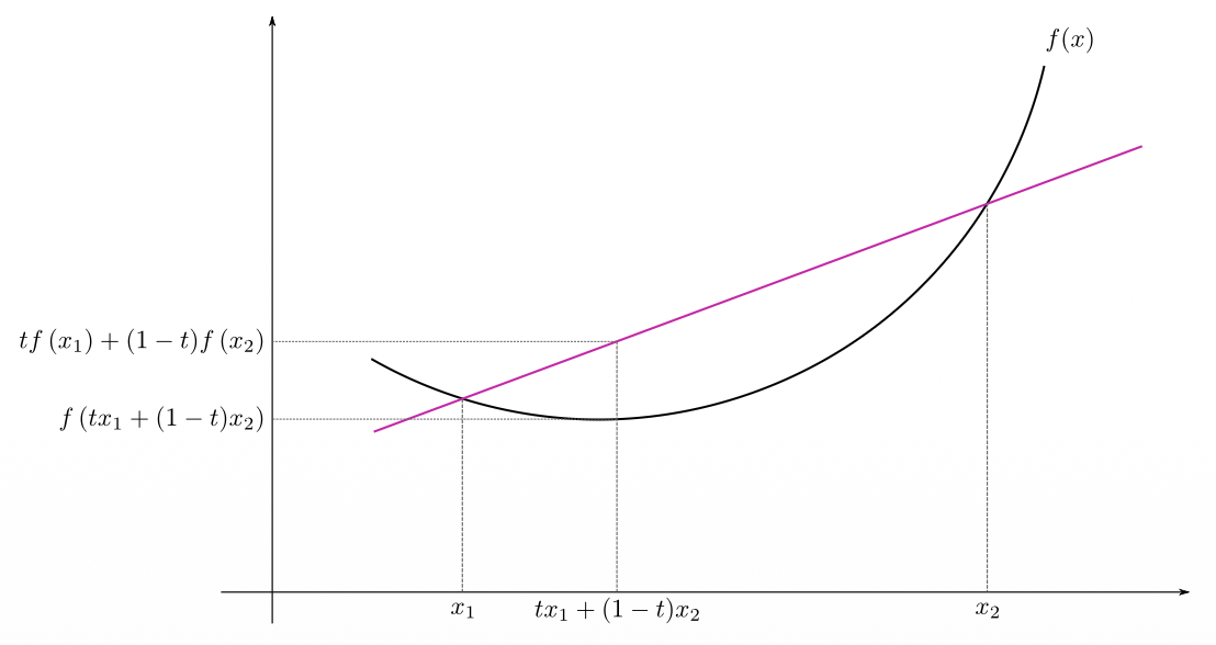
Convexity

(1) Mathematically, a function $f(\cdot )$ is convex if

(2) A function $f(\cdot )$ is strictly convex if

(3) Intuitively, a function is convex if the line segment between any two points on the function is not below the function.

(4) A function is strictly convex if the line segment between any two distinct points on the function is strictly above the function, except for the two points on the function itself.

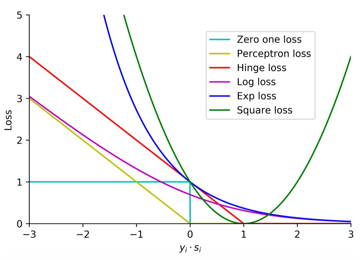
(5) In the zero-one loss, if a data sample is predicted correctly $(y_i{s}_i>0)$, it results in zero penalties; otherwise, there is a penalty of one. For any data sample that is not predicted correctly, it receives the same loss.

(6) For the perceptron loss, the penalty for each wrong prediction is proportional to the extent of violation. For other losses, a data sample can still incur penalty even if it is classified correctly.

(7) The log loss is similar to the hinge loss but it is a smooth function which can be optimized with the gradient descent method.

(8) While log loss grows slowly for negative values, exponential loss and square loss are more aggressive.

(9) Note that, in all of these loss functions, square loss will penalize correct predictions severely when the value of $y_i{s}_i$ is large.

(10) In addition, zero-one loss is not convex while the other loss functions are convex. Note that the hinge loss and perceptron loss are not strictly convex.

Notes:

• Convex functions look like that
• If you plot a straight line you can touch two points of the curve
• Convex:
  • the line segment between any two points on the function is not below the function
• Strictly convex:
  • the line segment between any two distinct points on the function is strictly above the function (except for the two points on the function itself)

Summary

• The key difference is from 0 to 1 and what happens if they are too close to the boundary.

• All of these are continuous except for the zero-one loss

• The log loss is especially differentiable at any point so that is why this is the one we use the most

• Convexity:

  • Zero-one: not convex
  • Perceptron: is convex but not strictly convex
  • Square loss: both convex and strictly convex
  • Log loss: both convex and strictly convex

• Continuous, differentiable and strictly convex functions are easier to optimize, this is why we use the log loss!

  • 90% of the time you will use Log loss
  • 9% of time you use Hinge loss
  • 1% the rest of the function (very specific cases)