05 - A Unified View of Loss Functions in Supervised Learning

Class: CSCE-421

Notes:

Intro

• So far we have only talk about two different loss functions and two different type of models, linear regression, and logistic regression.
• The loss is how you measure the difference between a predicted value and the real target (label)
  • In Linear regression we use least squares
  • In logistic regression we use the cross-entropy loss
• Today we will be dealing with a more general view of loss functions and other considerations

A Unified View of Loss Functions: Binary-Class Classifier

The Math

(1) Given a dataset $X=[{\mathrm{x}}_1,{\mathrm{x}}_2,\dots ,{\mathrm{x}}_n]$ with the corresponding label $Y=[y_1,y_2,\dots ,y_n]$, where ${\mathrm{x}}_i\in {\mathbb{R}}^{d+1}$ and $y_i\in \{+1,-1\}$.

• X is our input vector
• y is our labels vector
• Note this is a two-class (binary) predictor

(2) For a given sample ${\mathrm{x}}_i$, a linear classifier computes the linear score $s_i$ as

(3) We study the relations between loss values and $y_i{s}_i$ :

• Predict -1 if $s_i$ is negative
• Predict +1 if $s_i$ is positive
• ⟹ Prediction is correct if $y_i{s}_i>0$
• Prediction confidence is large if $\left|s_i\right|$ is large
• ⟹ Prediction is very correct if $y_i{s}_i\gg 0$
• ⟹ Prediction is very wrong if $y_i{s}_i\ll 0$

Notes:

• Our predictions are based on $s_i$
• If the $s_i$ is positive you predict (+1), otherwise (-1)
• Now after knowing our prediction we can put it the true label with the score. If these two are different, the prediction will be wrong, but if they are equal the prediction will be correct
  • Note both $y_i$ and $s_i$ need to be of the same sign to yield a correct prediction.
• If $s_i$ has a large magnitude, then the prediction confidence is large, you have a high score!
• Similarly,
  • if $y_i{s}_i$ is very positive (much larger than 0) you have a very confident prediction
  • if $y_i{s}_i$ is very negative (much smaller than 0) you have a very wrong prediction

The Meaning

1. The Magic Metric: $y_i{s}_i$ (The Agreement Score) Up until now, we have looked at different loss functions for different problems (Least Squares for Regression, Cross-Entropy for Logistic Regression). To create a "unified view" of all classification loss functions, we need a single mathematical way to represent how right or how wrong a model's prediction is.

We do this by combining two things:

• The true label ($y_i$): Either $+1$ or $-1$.
• The raw linear score ($s_i$): The raw dot product $s_i=w^T{x}_i$, which can be any number from $-\mathrm{\infty }$ to $+\mathrm{\infty }$.

When we multiply these together to get $y_i{s}_i$, it tells us everything we need to know about the prediction:

• The Sign (Correctness): If the true label $y_i$ and the score $s_i$ have the exact same sign (both positive or both negative), multiplying them together results in a positive number ($y_i{s}_i>0$). This means the model's prediction matches reality. If they have opposite signs, $y_i{s}_i<0$, meaning the model is wrong.
• The Magnitude (Confidence): The absolute value $|s_i|$ represents how far the data point is from the decision boundary. If it is a huge number, the model is highly confident.
  • $y_i{s}_i\gg 0$: The model is very confident and correct.
  • $y_i{s}_i\ll 0$: The model is very confident and wrong.

Zero-One Loss

The Math

(1) Prediction is correct if $y_i{s}_i>0$

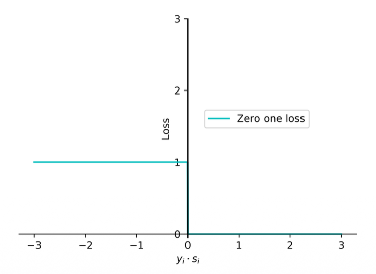
(2) The zero-one loss aims at measuring the number of prediction errors

(3) The loss for the entire training data is $\frac{1}{n}\sum _{i=1}^n{L}_{0/1}(y_i,s_i)$

Notes:

• The first loss function that we will talk about
• It will be 1 when $y_i{s}_i$ is negative and 0 if $y_i{s}_i$ is positive
• What does this loss do?
  • We know that any sample below $y_i{s}_i=0$ is wrong and above that is correct
  • This will just give you an n integer number of how many samples are mis-predicting
• If we want to minimize the training loss
  • If we use the zero-one loss we are just minimizing the number of wrong predictions
• This loss function is not commonly used because it is not continuous, you will have to deal with discrete optimization (since there is a jump from 0 to 1)
  • The cross-entropy loss is a continuous optimization of this functions

The Meaning

2. The Zero-One Loss ($L_{0/1}$) The Zero-One loss is the simplest, most intuitive way to measure error. It acts like a very strict teacher grading a test.

• If your prediction is correct ($y_i{s}_i\ge 0$), you get $0$ penalty points.
• If your prediction is wrong ($y_i{s}_i<0$), you get exactly $1$ penalty point.

To find the total error of your model on the whole dataset, you just average these penalties: $\frac{1}{n}\sum _{i=1}^n{L}_{0/1}(y_i,s_i)$.

The total Zero-One loss is literally just the percentage of misclassified examples in your dataset.

3. The Problem with Zero-One Loss Your final note highlights the most important takeaway: "This loss function is not commonly used because it is not continuous, you will have to deal with discrete optimization".

Why is this bad? Remember the analogy of Gradient Descent: a ball rolling down a smooth hill to find the minimum. If you graph the Zero-One loss, it is not a smooth hill. It is a perfectly flat line at $0$, and then a sudden, sharp vertical cliff jumping up to $1$. Because the line is completely flat everywhere except at the cliff, the gradient (slope) is exactly zero almost everywhere. If the computer tries to find the slope to figure out which way to step, it gets $0$, so it doesn't know how to adjust the weights.

To use Gradient Descent, we must replace this "stair-step" cliff with a smooth, curved approximation (like the Cross-Entropy Log Loss) that a computer can easily roll a ball down.

Perceptron loss

The Math

(1) The zero-one loss incurs the same loss value of 1 for all wrong predictions, no matter how far a wrong prediction is from the hyperplane.

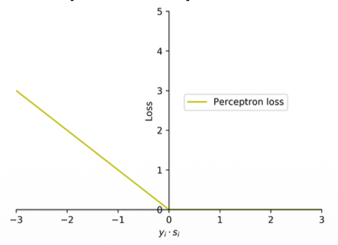
(2) The perceptron loss addresses this by penalizing each wrong prediction by the extent of violation. The perceptron loss function is defined as $\frac{1}{n}\sum _{i=1}^n{L}_p(y_i,s_i)$, where $L_p$ is perceptron loss which can be described as

(3) Note that the loss is 0 when the input example is correctly classified. The loss is proportional to a quantification of the extent of violation ( $-y_i{s}_i$ ) when the input example is incorrectly classified.

Notes:

• I f$y_i{s}_i$ is positive then you have a positive value as max, if $y_i{s}_i$ is negative then you will have a negative value as max?
• Somehow this loss seems to work right
• It will not give you the number of mis-predictions
• Is an approximation of the zero-one function

The Meaning

1. Perceptron Loss: Measuring "How Wrong" You Are In the previous slide, we saw that the Zero-One loss is flawed because it gives a flat penalty of $1$ for any mistake, whether the model was barely wrong or completely wrong. It also forms a "cliff" that prevents computers from using Gradient Descent (since the slope is $0$ everywhere else).

The Perceptron Loss fixes this by penalizing the model based on the extent of the violation.

• Fixing your note: You asked, "If $y_i{s}_i$ is positive then you have a positive value as max, if $y_i{s}_i$ is negative then you will have a negative value as max?" This is incorrect. Let's look closely at the formula: $L_p(y_i,s_i)=max(0,-y_i{s}_i)$. Notice the negative sign inside the function!
  • If your prediction is correct ($y_i{s}_i$ is a positive number, say $+5$), the formula becomes $max(0,-5)$. The maximum of $0$ and $-5$ is $0$. So, there is zero penalty for being correct.
  • If your prediction is wrong ($y_i{s}_i$ is a negative number, say $-5$), the negative sign flips it: $max(0,-(-5))=max(0,5)$. The maximum is $5$. The loss is $5$.
  • Therefore, the loss is never negative. It is exactly $0$ for correct predictions, and it scales up linearly (like a ramp) the further wrong a prediction is.

Because it forms a continuous ramp instead of a sharp cliff, the computer can now measure a slope and adjust the weights, making it a functional approximation of the Zero-One loss. However, while it is convex, it is not strictly convex (it doesn't form a perfect rounded bowl), which can sometimes make optimization slightly less smooth than other methods.

Square loss

The Math

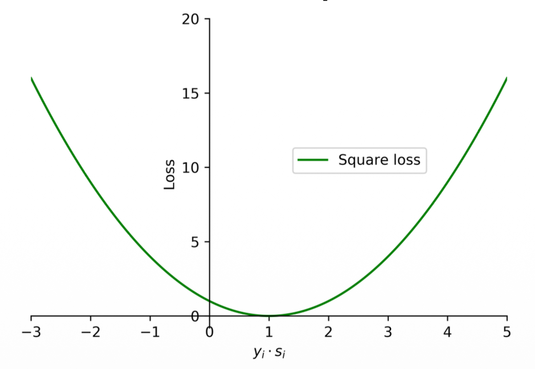
(1) The square loss function is commonly used for regression problems.

(2) It can also be used for binary classification problems as

where $L_s$ is the square loss, defined as

(3) Note that the square loss tends to penalize wrong predictions excessively. In addition, when the value of $y_i{s}_i$ is large and the classifier is making correct predictions, the square loss incurs a large loss value.

Notes:

• This will not perform well because whenever you have a correct prediction the loss will still be high!

The Meaning

Square Loss: The Danger of Being "Too Right" Next, the slide introduces the Square Loss: $L_s(y_i,s_i)=(1-y_i{s}_i{)}^2$. You already know this function—it is the standard error measure used for Linear Regression. However, this slide explores what happens if we blindly try to use it for classification.

• Fixing the note: "This will not perform well because whenever you have a correct prediction the loss will still be high!" This is close, but needs a slight correction. If $y_i{s}_i$ is exactly $1$, the loss is $(1-1{)}^2=0$. So it can be zero. The real problem is what happens when $y_i{s}_i$ is very large (e.g., $y_i{s}_i=10$). A large $y_i{s}_i$ means the model's prediction is both correct and extremely confident. If we plug $10$ into the formula: $(1-10{)}^2=(-9{)}^2=\mathbf{81}$.

This is the fatal flaw of using Square Loss for classification: it severely penalizes the model for being "too correct". Because it is a parabola (a U-shape), the penalty shoots up equally on both sides. The model will waste its time trying to pull its highly confident correct predictions back down to exactly $1$, rather than focusing on fixing its actual mistakes.

While Square Loss is perfectly smooth and strictly convex (making the math very easy), this over-penalization of correct predictions makes it a poor choice for classification tasks.

Log loss (cross entropy)

The Math

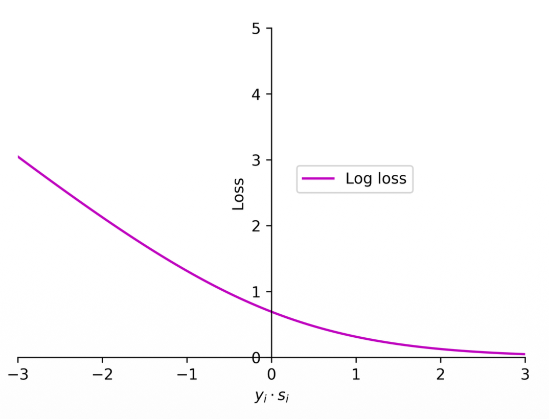
(1) Logistic regression employs the log loss (cross entropy) to train classifiers.

(2) The loss function used in logistic regression can be expressed as

where $L_{\text{log }}$ is the log loss, defined as

Notes:

• Note this is still some kind of approximation of the zero-one loss
• This is commonly used because it is a continuous function and differentiable everywhere
• What is the difference between Perceptron loss and cross entropy loss?
  • Should there be some loss close to 0 or not?
    • Yes, even though it is positive, it is small and represents a weak prediction even though it is correct, we can measure this with the Log loss by applying some loss closer to the 0 boundary
    • The Log loss basically makes it so that the bigger the number (positive) the less the loss.
  • The cross entropy loss is differentiable!
  • For logistic regression there is no perfect sample, every sample has some loss
    • For strong predictions this value would be very small but never will be zero
    • This is because of how logs work (horizontal asymptote at 0)

The Meaning

1. Log Loss (Cross Entropy) is perfectly smooth and everywhere differentiable. It forms a perfect, rounded bowl (it is strictly convex), which is exactly why we love using it for Gradient Descent.

• It is the Perceptron Loss and the Hinge Loss that have a "sharp edge" (a non-differentiable point where the line suddenly hinges like a bent knee).

2. Log Loss: Never satisfied, always pushing You asked in your notes: "Should there be some loss close to 0 or not?" The answer is yes! If $y_i{s}_i$ is positive but very small (e.g., $0.05$), it means the model guessed correctly, but it is extremely unconfident.

• The Perceptron Loss stops caring the absolute millisecond the prediction is correct ($y_i{s}_i>0$). It assigns $0$ penalty.
• The Log Loss realizes that a weak prediction is dangerous. Because of the horizontal asymptote of the log function, the loss never truly reaches exactly zero. It continuously applies a tiny penalty to correct predictions, forcing the algorithm to push the weights to be as confident as possible.

Hinge loss (support vector machines)

The Math

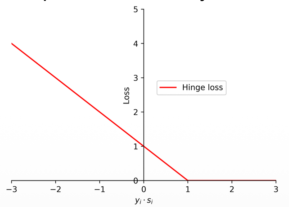
(1) The support vector machines employ hinge loss to obtain a classifier with "maximum-margin".

(2) The loss function in support vector machines is defined as follows:

where $L_h$ is the hinge loss:

(3) Different with the zero-one loss and perceptron loss, a data may be penalized even if it is predicted correctly.

Notes:

• Differences of the Hinge loss
  • Note the difference from perceptron loss:
    • Perceptron loss: $max(0,-y_i{s}_i)$
    • Hinge loss: $max(0,1-y_i{s}_i)$
  • The only difference is that 1, and it has a significant impact
    • Essentially it shifts the curve by 1.
    • This applies some loss for the positive predictions closer to 0, like the log loss
    • But still is not a differentiable function
  • Note the log loss would still be a little bit more harsh on positive predictions closer to 0 (applies a bit more loss)
  • The reason we use this is because it could be the case that fits better our data helping the maximum margin (the distance between the loss line and the data points)
    • The reason it is called maximum margin is because of that small loss that applies to weak correct predictions
• Support and non-support vectors:
  • If a data point has zero loss, if you remove this data point, and re-train, the model will remain the same.
    • These are called non-support vectors (points that if removed, the model will remain the same)
    • The other data points are support vectors (incorrect predictions and closer to 0 correct predictions)
    • Look for a visual example of support and non-support vectors
      • To distinguish these two is not trivial, because you need to identify all the data points and how the maximum margin would change if removed
• Something interesting:
  • Why is it 1? Why shifting by 1? is there any difference if we put a 5 there? What would be the difference?
  • If you make it 0 it will just care about if predictions are correct or not (just like perceptron)
  • If you use any positive number the effect will be the same!
    • Regardless of by how many you scale, the margin will remain the same
    • You can use any number! It is just a scale.
  • The only reason that this loss is not really used in deep learning is because it only works for two classes.

The Meaning

3. Hinge Loss: Demanding a "Margin" of Safety The Support Vector Machine (SVM) uses Hinge Loss: $L_h(y_i,s_i)=max(0,1-y_i{s}_i)$. You perfectly noticed the only difference between this and Perceptron loss is the shift by 1. This 1 has a massive impact.

• Instead of just asking to be barely correct ($y_i{s}_i>0$), Hinge Loss demands a margin of safety. It penalizes the model until the confidence score is strictly greater than or equal to $1$ ($y_i{s}_i\ge 1$).
• If the model gets the answer right but the score is only $0.5$, Hinge Loss still applies a penalty of $0.5$. It forces the model to push the data points away from the boundary until they are safely past the $1$ threshold.

4. Support vs. Non-Support Vectors Because Hinge Loss becomes exactly zero once $y_i{s}_i\ge 1$, an interesting phenomenon occurs.

• Non-Support Vectors: Any data point that is correctly classified and safely outside the margin ($y_i{s}_i\ge 1$) has $0$ loss. If you completely delete these points from your training dataset and retrain the model, the decision boundary will not move a single inch.
• Support Vectors: The model's boundary is entirely propped up (supported) by the points that are inside the margin, on the margin edge, or completely misclassified. These are the only points the algorithm cares about.

5. "Why is it 1? Can we use 5?" Your intuition here is incredibly sharp and correct! If you used $max(0,5-y_i{s}_i)$, the algorithm would just scale the entire weight vector $w$ up by a factor of 5 to achieve the exact same geometric separating line. The margin would look the same relative to the data. We use $1$ simply because it is the cleanest mathematical standard to anchor the scale.

6. Why deep learning prefers Log Loss Your note suggests Hinge Loss isn't used in Deep Learning because it only works for two classes. While multi-class adaptations of Hinge Loss do exist, the real reason Deep Learning universally prefers Log Loss is back to your first note: Differentiability and Probabilities. Log loss is completely smooth (easy for backpropagation/gradient descent) and pairs perfectly with the Softmax function to output clean percentages (probabilities), whereas Hinge Loss just outputs raw, hard boundary scores.

Exponential Loss

The Math

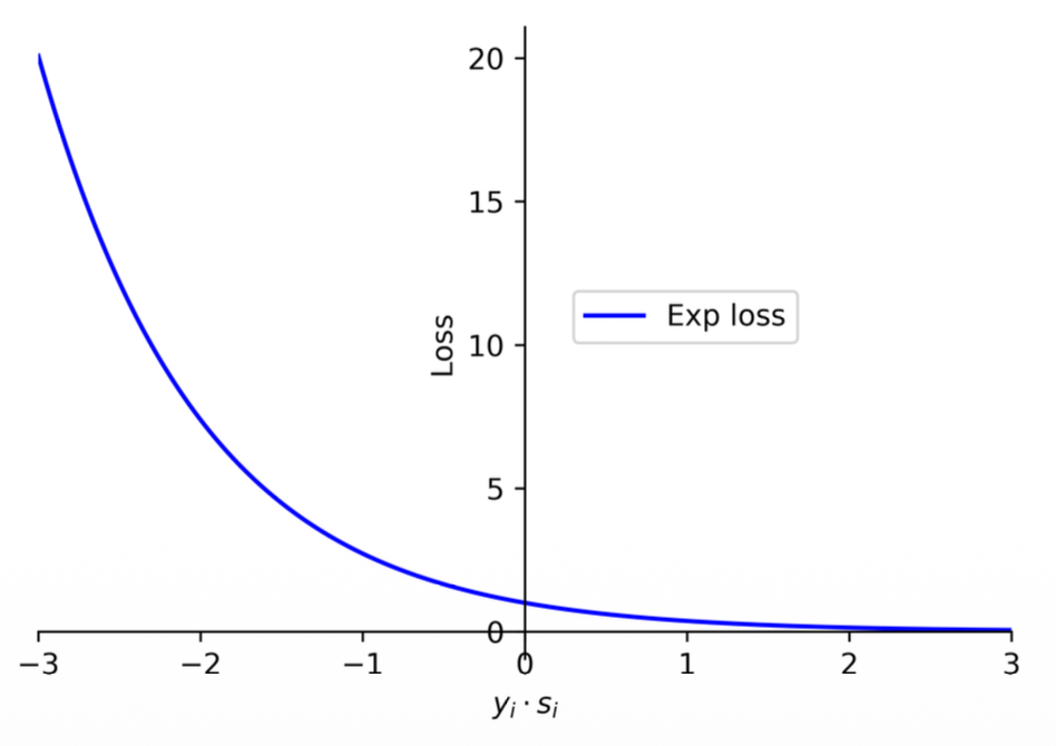
(1) The log term in the log loss encourages the loss to grow slowly for negative values, making it less sensitive to wrong predictions.

(2) There is a more aggressive loss function, known as the exponential loss, which grows exponentially for negative values and is thus very sensitive to wrong predictions. The AdaBoost algorithm employs the exponential loss to train the models.

(3) The exponential loss function can be expressed as $\frac{1}{n}\sum _{i=1}^n{L}_{\exp }(y_i,s_i)$, where $L_{\text{exp }}$ is the exponential loss, defined as

Notes:

• Some commercial models and libraries use this loss
• It penalizes data points that are wrong and be a little bit more permissive in correct predictions closer to 0.

The Meaning

Exponential Loss: The "Aggressive" Metric The formula for Exponential Loss is $L_{exp}(y_i,s_i)=e^{-y_i{s}_i}$. To understand why your slide calls it "aggressive," let's compare it to the Perceptron and Log losses when the model makes a very wrong prediction (e.g., $y_i{s}_i=-5$):

• Perceptron Loss: $max(0,-(-5))=\mathbf{5}$.
• Log Loss: $\log (1+e^5)\approx \mathbf{5.006}$.
• Exponential Loss: $e^5\approx \mathbf{148.4}$.

As you can see, Exponential Loss punishes wrong predictions astronomically! If even a single data point is misclassified by a large margin, the error skyrockets. This forces the learning algorithm to focus intensely on fixing its biggest mistakes. This is the exact mathematical engine that powers AdaBoost (a famous algorithm that builds classifiers by obsessively focusing on the hardest-to-classify data points).

• Note on your notes: "a little bit more permissive in correct predictions closer to 0". Actually, its main defining trait is how extremely un-permissive it is to negative numbers (wrong predictions). For correct predictions, it smoothly decays to $0$ as confidence grows, much like log loss.

Convexity

The Math

(1) Mathematically, a function $f(\cdot )$ is convex if

(2) A function $f(\cdot )$ is strictly convex if

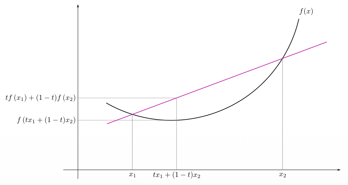
(3) Intuitively, a function is convex if the line segment between any two points on the function is not below the function.

(4) A function is strictly convex if the line segment between any two distinct points on the function is strictly above the function, except for the two points on the function itself.

(5) In the zero-one loss, if a data sample is predicted correctly $(y_i{s}_i>0)$, it results in zero penalties; otherwise, there is a penalty of one. For any data sample that is not predicted correctly, it receives the same loss.

(6) For the perceptron loss, the penalty for each wrong prediction is proportional to the extent of violation. For other losses, a data sample can still incur penalty even if it is classified correctly.

(7) The log loss is similar to the hinge loss but it is a smooth function which can be optimized with the gradient descent method.

(8) While log loss grows slowly for negative values, exponential loss and square loss are more aggressive.

(9) Note that, in all of these loss functions, square loss will penalize correct predictions severely when the value of $y_i{s}_i$ is large.

(10) In addition, zero-one loss is not convex while the other loss functions are convex. Note that the hinge loss and perceptron loss are not strictly convex.

Notes:

• Convex functions look like that
• If you plot a straight line you can touch two points of the curve
• Convex:
  • the line segment between any two points on the function is not below the function
• Strictly convex:
  • the line segment between any two distinct points on the function is strictly above the function (except for the two points on the function itself)

The Meaning

1. Convexity: The Mathematics of a "Bowl" You already know intuitively that a convex function looks like a bowl, which is great for Gradient Descent. The slide provides the formal mathematical proof of what a "bowl" is: $$f(t x_1 + (1-t) x_2) \leq t f(x_1) + (1-t) f(x_2)$$ Let's translate this math into English:

• Imagine picking two points on the curve, $x_1$ and $x_2$.
• The term $t{x}_1+(1-t)x_2$ just means "choose an $x$-coordinate somewhere exactly between $x_1$ and $x_2$."
• The left side of the equation ($f(\dots )$) is the actual curve of the function at that middle point.
• The right side of the equation is a straight line drawn between the two points.
• The formula simply says: "The curve must always dip below (or equal) the straight line." If you draw a line across the top of a bowl, the bottom of the bowl is always beneath the line!

2. Convex vs. Strictly Convex Why do we care about "Strictly" convex?

• Convex ( $\le$ ): The curve can dip below the line, or it can be perfectly flat and equal the line. The Perceptron Loss and Hinge Loss are V-shaped or have flat sections. They are convex, meaning a rolling ball won't get trapped in a fake local minimum, but because of the flat parts, the ball might stop rolling on a flat "plateau" (a valley floor) instead of a single perfect point.
• Strictly Convex ( $<$ ): The curve strictly dips below the line. There are absolutely no flat parts. Square Loss, Log Loss, and Exponential Loss are strictly convex. This guarantees there is exactly one unique, perfect global minimum at the very bottom of a rounded bowl.

Summary

• The key difference is from 0 to 1 and what happens if they are too close to the boundary.

• All of these are continuous except for the zero-one loss

• The log loss is especially differentiable at any point so that is why this is the one we use the most

• Convexity:

  • Zero-one: not convex
  • Perceptron: is convex but not strictly convex
  • Square loss: both convex and strictly convex
  • Log loss: both convex and strictly convex

• Continuous, differentiable and strictly convex functions are easier to optimize, this is why we use the log loss!

  • 90% of the time you will use Log loss
  • 9% of time you use Hinge loss
  • 1% the rest of the function (very specific cases)

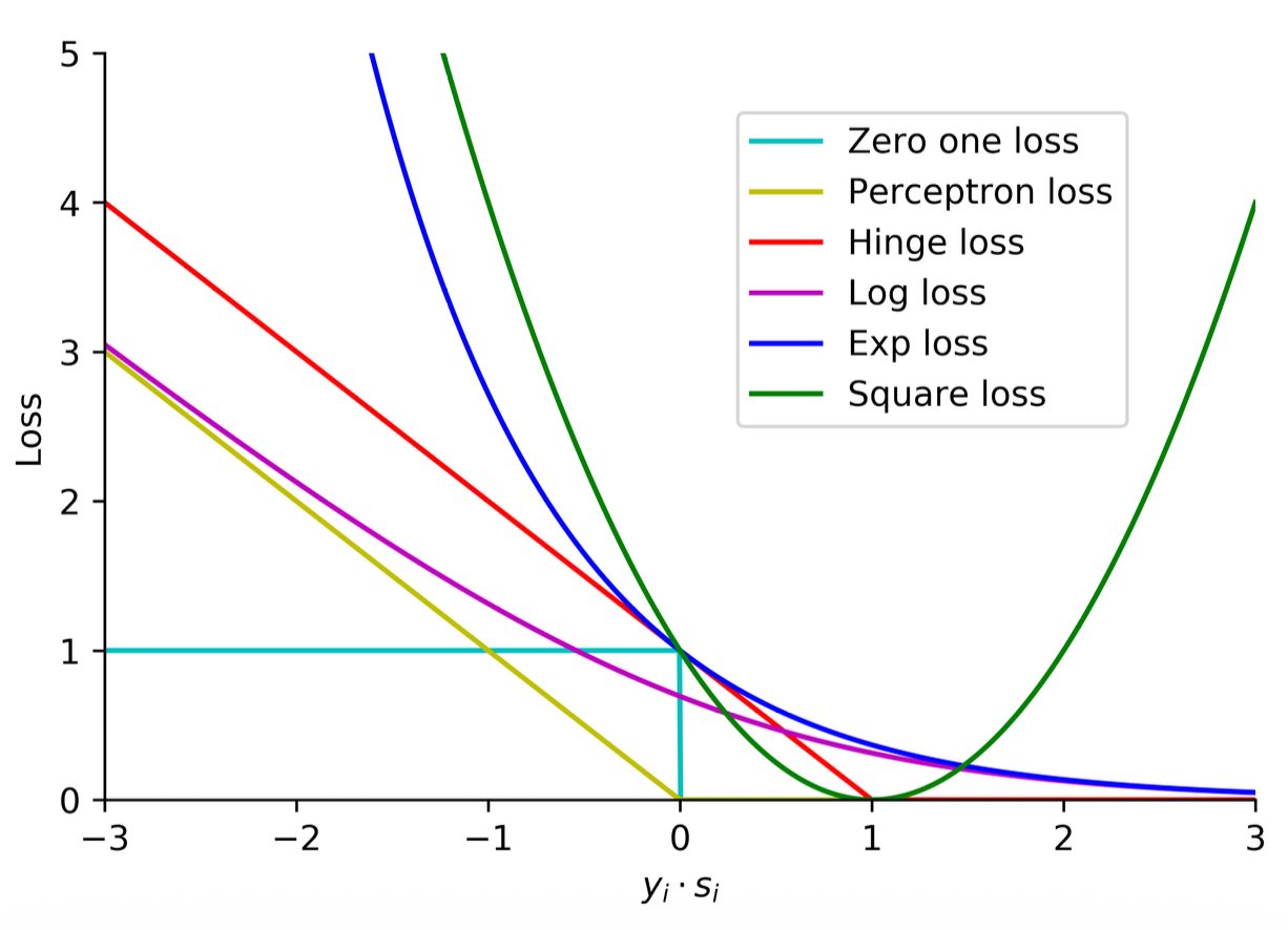
The Grand Summary of Loss Functions The end of your slide brilliantly summarizes everything you need to know for choosing a loss function:

• Zero-One Loss: Perfect in theory (counts exact errors), but impossible to optimize because it is a flat stair-step (not convex, not differentiable).
• Square Loss: Perfectly smooth and strictly convex, but terrible for classification because it severely penalizes the model for being "too correct" ($y_i{s}_i\gg 0$).
• Perceptron & Hinge Loss: Convex, but not strictly convex (they have sharp corners/flat edges). Good for finding margins, but you can't always use simple Gradient Descent easily on the sharp corners.
• Log Loss: The Goldilocks function. It is continuous, everywhere differentiable, and strictly convex. It smoothly pushes correct predictions to be more confident. This is why it is the absolute standard for Logistic Regression and Deep Learning.
• Exponential Loss: Also smooth and strictly convex, but highly aggressive. It is used specifically when you want an algorithm (like AdaBoost) to fiercely penalize errors.