10 - Attention, Transformers, and Large Language Models

Class: CSCE-421

Notes:

These slides are based on Chapter 12 of Deep Learning: Foundations and Concepts

Word Embedding

Example

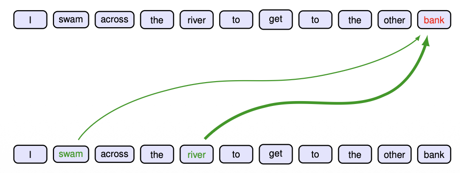
I swam across the river to get to the other bank.
I walked across the road to get cash from the bank.

• Appropriate interpretation of 'bank' relies on other words from the rest of the sequence
• The particular locations that should receive more attention depend on the input sequence itself
• In a standard neural network, the weights are fixed once the network is trained
• Attention uses weights whose values depend on the specific input data

Notes:

• How do we deal with sentences-words?
• The meaning of a word sometimes depends on the context, this is the key idea that LLMs work around.
• Imagine you have a sentence like the above
  • I will somehow process and match each of these words into a vector
    • The vector needs to be of the same dimension of course
  • Then you will have a sequence of vectors, with each vector representing a word, then you will produce a sequence of vectors as outputs, and you will do this in many layers.
  • The key operation is that you have a sequence of words, equivalent to a sequence of vectors and you can transform this into a sequence of vectors as output.
• We want to transform from the input vectors to the output vectors
  • The number of words in this unit cannot change!
  • If you have 10 vectors as input, your output will be 10 vectors
  • Across different layers, the number of layers can change but the number of vectors cannot.
  • The key idea here is: if the input vectors are given, how do we get the output vectors?
• If you want this vectors to capture semantics, what do we need to do?
  • The vector for a specific word has to deppend in many input vectors
  • To compute each of these output vectors will depend on all of the input vectors
  • Each of the output vectors will be a linear combination of the input vectors
  • Which one is more important? we do not worry about that, that is learnt in training.
  • This is the idea of Attention: pay different attention to different inputs with different weights
• First how can we convert a word into a vector?
  • The first layer needs to convert each of the words into a vector
  • This layer is called the embedding layer
  • There is a very simple way: one-hot representation
  • Lets say there are 50,000 words in English, now you have a vocabulary, each word has an index in that vocabulary (a fixed number in that vocabulary), then you can convert each of this words into a vector of 50,000 thousand dimensions, with the single index entry corresponding to the word is 1, and all the other entries are 0.
• Note each vector will correspond to a word, and therefore the number of vectors cannot change
  • But your network needs to be able to take different input sizes
• Most discussions: given a sequence of vectors, how do you produce another sequence of vectors. This is also called Attention

Neural language and word embedding

• Convert the words into a numerical representation that is suitable for use as the input to a deep neural network
• Define a fixed dictionary of words and then introduce vectors of length equal to the size of the dictionary along with a 'one hot' representation for each word
• The embedding process can be defined by a matrix E of size $D\times K$ where $D$ is the dimensionality of the embedding space and $K$ is the dimensionality of the dictionary.
• For each one-hot encoded input vector ${\mathrm{x}}_n$ we can then calculate the corresponding embedding vector using

• Word embeddings can be viewed as the first layer in a deep neural network. They can be fixed using some standard pre-trained embedding matrix, or they can be trained
• The embedding layer can be initialized either using random weight values or using a standard embedding matrix

Notes:

• Understand the equation:
  • $x_n$ is a one-hot representation vector of the word. (Each of these words are a one-hot vector) The dimension of this vector is the number of words in the vocabulary.
    • One location that has a value of 1, and every other location has a value of 0.
    • You can use it but this might not be a good representation, just because it is a extremely long vector containing all 0s but a 1.
  • What you do is multiply the matrix $E$ (${\mathrm{v}}_n={\mathrm{Ex}}_n$).
    • Remember matrix multiplication is a linear combination of columns
    • By far the most important operation in linear algebra matrix-vector multiplication
    • You multiply each element on the vector to each of the columns and sum them together.
    • You basically take a particular column of this matrix because all entries on $x_n$ are 0, except for the word entry.
    • You are basically converting a long vector into a shorter vector
    • $E$ is learned, and is called the embedding matrix.
  • The output will be $v_n$, it is the vector that we used as the input to the next layer for process.
  • This is nothing but a fully connected network thanks to a matrix multiplication, we are applying a fully connected network to every location of the input (every word vector) - one applied for each word separately.
• A little bit more context:
  • Imagine you have the previous sequence of words. Intuitively your first step is to convert each word into its one-hot English representation.
    • You will then have $x_1,x_2,\cdots ,x_n$
    • Then your output vectors would look like: $v_1,v_2,\cdots ,v_n$
  • The operation in between is matrix-multiply with $E$.
    • But what is this operation in terms of neural networks? (use neural network terminology - not mathematically)
      • It is forward propagation? yes
      • We are talking about a fully connected layer? yes, but there is something else...
      • This is nothing but a neural network layer that you already know
      • But what else is $E$?
        • You have one fully connected layer that is shared across all the words, it is a single $E$.
        • A fully connected network
        • The key is that the same network is applied to each of the input vectors.
        • This is simply a fully connected layer but shared among all the input vectors.
• Exam question: Explain the embedding layer from a neural network point of view.
  • -> fully connected layer shared among all the input vectors
• But this is just the first layer!

Checkpoint 1 (word embedding)

To understand Large Language Models (LLMs) like ChatGPT, we have to start at the very beginning: How do we teach a neural network to read words, and how do we teach it to understand context?

1. The "Context" Problem (The Example) Read these two sentences:

• "I swam across the river to get to the other bank."
• "I walked across the road to get cash from the bank."

As a human, you instantly know the word "bank" means two completely different things here. You know this because you subconsciously looked at the surrounding words ("river" and "swam" vs. "cash"). In a standard Neural Network (like a CNN or MLP), the weights are permanently fixed after training. If you feed it the word "bank," it will always process it using the exact same fixed weights, completely ignoring the unique context of the sentence.

2. The Solution: Attention To solve this, we need a network that can change its weights on the fly depending on the specific sentence it is reading. This is called Attention. In an Attention layer, when the network is trying to process the word "bank," it dynamically calculates a set of weighting coefficients that determine how much "attention" it should pay to every other word in the sentence. In the first sentence, it will assign a massive mathematical weight to the word "river", effectively blending the meaning of "river" into "bank".

• The Core Rule: An Attention layer takes a sequence of input vectors and produces a sequence of output vectors. The number of vectors does not change. If you input 10 words, you output 10 transformed words. Every single output vector is calculated as a linear combination of all the input vectors.

3. Neural Language & Word Embeddings Before we can even do Attention, we have to convert English words into numbers, because neural networks can only do math. This happens in the very first layer of the network, called the Embedding Layer.

• Step A: The One-Hot Vector ($x_n$) Imagine a dictionary of 50,000 English words. We can represent the word "apple" as a massive vector consisting of 50,000 numbers. The index corresponding to "apple" is set to 1, and the other 49,999 numbers are set to 0. This is called a one-hot vector ($x_n$).
• Step B: The Embedding Matrix ($E$) A 50,000-dimensional vector of mostly zeros is completely useless and computationally heavy. We want to compress it into a short, dense vector of meaningful numbers (say, 300 dimensions). To do this, we create a massive weight matrix called $E$ (with $D=300$ rows and $K=50,000$ columns).
• Step C: The Math ($v_n=E{x}_n$) We multiply our massive $E$ matrix by our one-hot vector $x_n$. Because $x_n$ is entirely zeros except for a single 1, the matrix multiplication essentially just acts as a "lookup table." It plucks out one specific column from the $E$ matrix and returns it as our new, short, 300-dimensional vector ($v_n$). This $v_n$ vector is what actually gets passed into the Attention layers!

4. The Neural Network View (EXAM QUESTION WARNING!) Your professor explicitly mentioned an exam question here: "Explain the embedding layer from a neural network point of view." Mathematically, doing $v_n=E{x}_n$ is the exact same formula as passing data through a standard Fully Connected layer ($w^{T}x$). However, because we use the exact same $E$ matrix to transform every single word in our sentence, the answer your professor is looking for is: An embedding layer is a fully connected layer that is shared among all the input vectors.

Attention

Transformer processing

The input data to a transformer is a set of vectors $\left\{x_n\right\}$ of dimensionality $D$, where $n=1,\dots ,N$

• Combine the data vectors into a matrix X of dimensions $N\times D$ in which the $n$th row comprises the token vector ${\mathrm{x}}_n^{\mathrm{T}}$, and where $n=1,\dots ,N$ labels the rows
• A Transformer takes a data matrix as input and creates a transformed matrix $\tilde{\mathrm{X}}$ of the same dimensionality as the output
• We can write this function in the form

Notes:

• This is the data in a particular layer
• For now, think of each token as a word.
• If you have 5 words, you will have 5 vectors in the matrix X
• We need to be able to take this X matrix and transform it into $\tilde{X}$
• Inside this layer the vectors have to be the same dimensions, otherwise we can not put this into a matrix.
• So now the question is given a matrix, how can we produce a new matrix.

Attention coefficients

• Map input tokens $x_1,\dots ,x_N$ to $y_1,\dots ,y_N$
• The value of $y_n$ should depend on all the vectors $x_1,\dots ,x_N$
• Dependence should be stronger for important inputs
• Define each output vector ${\mathrm{y}}_n$ to be a linear combination of ${\mathrm{x}}_1,\dots ,{\mathrm{x}}_N$ :

where

Commonly used coefficients

We have a different set of coefficients for each output vector $y_n$

Notes:

• input sequence: x1,...,xn (each of these is a vector)
  • the number of vectors cannot change
• output sequence: y1,...,yn
  • each of these outputs depend on all the input vectors
  • (will be a linear combination of each of the input vectors)
  • More important ones will be given a larger weight, less important ones are given a smaller weight.
• Note $a_{nm}$ is just in linear combination with $x_m$ for a particular $y_n$
  • This is a coefficient, and summing all of them will give 1.
  • The whole idea here is that through this entire network the number of vectors will not change.
• Attention is basically is how to get $a_{nm}$
  • We are trying to compute $y_n$ because if we can do this for one vector, we can do it for all of them
    • All we need is $a_{nm}$ where $a_n=[a_{n_1},a_{n_2},...,a_{n_N}{]}^T$
  • Lets say we are computing this coefficient, how?
    • You will take your $x_n$ and take its product with each of the $x_1,x_2,...,x_N$
    • The output will sum to 1, and every coefficient will be between 0 and 1.

Attention in general (cross attention) - IMPORTANT

• Use of query, key, and value vectors as rows of matrices Q,K,V

Notes:

• We are defining a more general attention operation, for this we introduce the general Q, K, V.
• Attention: In the most general case, the attention operation will take 3 sequences of vectors as inputs and produce 1 sequence of vectors as output.
  • Q (sequence of vectors)
  • K (sequence of vectors)
  • V (sequence of vectors)
• Self attention:
  • Where Q = K = V = X (generally)
  • You can always give Q, K, V the same things, but you are better giving something more useful
• The question is: How to produce one vector in the output.
  • You take an arbitrary row in Q, and produce a sequence of vectors for that row.
  • We will take the pink vector in Q, then do an inner product of this vector and each rows of K,
  • Then this vector is passed through Softmax to get another vector (converting to [0,1] and sum to 1).
    • It turns out if you give Q, K, V the same x, this will be just 1.
  • Then you again do an inner product of this vector with all rows on V to get the final one vector sequence.
• Question: The sizes of Q, K, V cannot be arbitrary, otherwise these operations won't work. But in general they do not have to be exactly the same size, but there has to be some kind of constraint for this to work.
  • The inner product is matrix multiplication of K^T so we need the same number of columns on Q and K.
    • Not necessarily same number of rows because we are either way takin each row on Q and inner product it with each row on K. They do not necessarily need to match.
    • Size of the cross vector will equal to the number of rows in K.
    • Softmax will not change the size.
  • K and V need to have the same number of rows, in order for each number to have a cross product.
• Question: How about the size of this output vector sequence?
  • We want to know how the size of the output relates to the size of the input
    • We will put this sequence of vectors into a matrix.
    • We want to know how many vectors are produced, and what is the size of each vector
  • The number of columns of each vector in this sequence needs to be the same as the number of columns in V.
    • Dimensions haves to equal in order to do the cross product
  • Now how many vectors?
    • The number of rows in Q?
• Question: If we permute rows in certain way, how the output will be changed?
  • Rows will also be permuted, because each row will be computed separately.
  • Moving a row in Q will just move the row in the output sequence.
  • What kind of property is this?
    • If you swap certain row, is equivalent to swapping certain words!
    • This is called permutation equivariance
    • It has a very important consequence in language models
    • If you change the order of the inputs, it will change the order of the outputs.
    • In natural languages this is not desired, because different order of words mean different things, so we need to do something else?
      • An answer will just be a permuted version of a prompt, which is not what we want.
• Question: What happens if we permute the rows in K and V (they have the same number of rows) using the same permutation, how the output would be changed?
  • It won't change!
  • It would only change if we permute one of them without permuting the other one.
  • This is because we use the a vector of Q to compute each of the cross products for each vector in K, since we have the same order in V because we also permuted it as K, then everything will remain the same.
• Note the most common case of this setup is for each of these Q, K, V to be the same matrix
  • This is called the self potential.
  • If my X is permuted, all of the Q, K, V will be permuted the same way
    • This means that the output will change because of Q being permuted
    • But the output remains in that way (after being permuted by Q) when applying K and V (those do not change the output).
• There is still a little bit something we need to do before, but for now this is the model
  • Do you think this will work in LLMs as of right now? NO
    • We haven't learned anything, we cannot train yet!
  • But there is a small step to make it work, we need to introduce some learning parameter.
• We can put all of this operations into a Matrix Form!

Checkpoint 2 (Attention in general)

To understand Large Language Models, we have to understand the core engine inside them: the Transformer layer and its Attention mechanism.

1. Transformer Processing Imagine a sentence with $N$ words (tokens). From the previous slides, we know the Embedding Layer converts each of these words into a vector of numbers of size $D$.

• If we stack all these $N$ vectors on top of each other, we get a massive input data matrix called $X$, which has dimensions $N\times D$ (Number of words $\times$ Dimensionality of each word).
• A Transformer Layer simply takes this matrix $X$ and transforms it into a brand new matrix $\tilde{X}$.
• The Golden Rule: The output matrix $\tilde{X}$ is the exact same size ($N\times D$) as the input. If you input 10 words, you get 10 "smarter, context-aware" words out.

2. Attention Coefficients How does the network make these word vectors "smarter"? It uses a linear combination. To generate the new output vector for the first word ($y_1$), the network looks at all the input vectors ($x_1,x_2,\dots ,x_N$) and blends them together.

• But how much of $x_2$ should be blended into $y_1$? That is determined by the attention coefficient ($a_{nm}$).
• Think of $a_{nm}$ as a percentage. All the coefficients for a specific output word must be non-negative and sum perfectly to $1$ (100%).
• How do we calculate these percentages? We take the dot product (which is the mathematical way to measure similarity) between the word we are currently processing and every other word in the sentence. Then, we pass those raw similarity scores through a Softmax function. As you learned in Logistic Regression, Softmax perfectly converts raw numbers into a probability distribution that sums to 1.

3. Attention in general (Q, K, V) - IMPORTANT This is the most critical concept. Calculating attention just by comparing $X$ to $X$ is a bit rigid. To make the network highly flexible, we introduce a database-like retrieval system using three matrices: Queries (Q), Keys (K), and Values (V). Think of a video streaming search:

• Query (Q): What you type into the search bar (e.g., "Funny cat").
• Key (K): The hidden tags attached to the videos in the database (e.g., "Comedy, Animal").
• Value (V): The actual video file you get to watch.

In neural networks:

1. You take a Query vector (the word you are currently trying to process) and calculate the dot product with every single Key vector (every other word's tags).
2. You apply Softmax to those scores to find out which Keys best match your Query (this gives you your coefficients).
3. You multiply those coefficients by the Value vectors to get your final output. (Note: In "Self-Attention", Q, K, and V are all just the input matrix $X$ itself, meaning the sentence is searching itself for context!).

4. The Rules of Q, K, V (Exam Warning!) Your professor highlighted specific exam questions regarding the dimensions and permutations of these matrices:

• Dimensions: You calculate the similarity by taking the inner product (matrix multiplication) of $Q$ and $K^T$. Because of how matrix math works, Q and K must have the exact same number of columns. Meanwhile, because every Key must correspond to a Value, K and V must have the exact same number of rows.
• Output Size: The final output matrix will have the same number of rows as $Q$ (because you get one output for every query) and the same number of columns as $V$ (because the output is made of value vectors).
• Permutation Equivariance: If you swap the order of the rows in $Q$ (e.g., swapping the 1st and 3rd words in your sentence), the output matrix simply swaps its 1st and 3rd rows. However, if you swap the rows in $K$ and $V$ in the exact same way, the output does not change at all. Why? Because the Query is still finding the exact same Keys and extracting the exact same Values, regardless of where they are physically located in the database!

Let's break down the exact math behind general attention from scratch so you can confidently put it on your cheat sheet. Your 3-step logic is actually perfectly correct conceptually, but it is missing the specific linear algebra rules that make it work.

Here is the detailed, step-by-step breakdown of how the matrices operate, why we use rows, and how the sizes are calculated.

1. What are "Rows"?

In Transformers, data is structured as a matrix where each row represents a single word (or token), and the columns are the numerical features (the embedding dimensions) of that word. Therefore, when we talk about $Q$, $K$, and $V$ matrices, we are looking at stacks of words. A single "$Q$ vector" is just one row from the $Q$ matrix, representing the specific "Query" word you are currently trying to process.

2. Step 1: The Dot Product ($Q{K}^T$)

You want to know how similar your single Query word (a row in $Q$) is to every single Key word (the rows in $K$). The mathematical way to measure similarity between two vectors is the dot product.

• The Math: In linear algebra, to multiply a row of numbers by another row of numbers, you must flip the second row into a column. This is why the attention formula uses $K^T$ (the transpose of $K$). Transposing $K$ turns all of its word-rows into columns.
• The Result: When you multiply your single $Q$ row by the entire $K^T$ matrix, you are computing the dot product between your query word and every single key word simultaneously. This outputs a single row vector of raw scalars, which are the similarity scores for that specific query word against all the keys.

3. Step 2: Softmax

You apply the Softmax function to that single row vector of raw scores. Softmax simply converts these numbers into a probability distribution—it turns them into a row of percentages (coefficients) between 0 and 1 that sum perfectly to 1.

4. Step 3: Multiplying by $V$

This is where the linear algebra magic happens. You now have a row vector of percentages, and you need to multiply it by the $V$ matrix (where each row is a Value word).

• The Math: According to the fundamental rules of linear algebra, multiplying a row vector by a matrix results in a linear combination of the rows of that matrix.
• The Result: The math automatically takes your percentages, scales each corresponding row in $V$ by its assigned percentage, and adds them all together into one single new vector. This single resulting vector is your final, context-aware output for the query word you started with.

5. What is the size of the final output?

Instead of processing one query word at a time, the equation $Y=\text{Softmax}[Q{K}^T]V$ processes all query words at once using matrix multiplication. Here is how the dimensions determine the final output size:

• The Rules: To perform these matrix multiplications, $Q$ and $K$ must have the exact same number of columns (so the dot product works), and $K$ and $V$ must have the exact same number of rows (because every Key must map to a Value).
• The Dimensions:
  • Let $Q$ have $N_Q$ rows (number of query words).
  • Let $K$ have $N_K$ rows (number of key words).
  • Let $V$ have $D_V$ columns (the feature dimension of the values).
• The Output Size: When you multiply the entire $Q$ matrix by $K^T$, the resulting Softmax score matrix is of size $N_Q\times N_K$ (every query word scored against every key word). When you multiply this $N_Q\times N_K$ score matrix by the $N_K\times D_V$ Value matrix, the inner dimensions ($N_K$) cancel out.
• The Final Size: The final output matrix $Y$ will have the same number of rows as $Q$, and the same number of columns as $V$.

General attention in matrix form

• The attention computes

where Softmax $[L]$ takes the exponential of every element of $L$ and then normalizes each row independently to sum to one

• Whereas standard networks multiply activations by fixed weights, here the activations are multiplied by the data-dependent attention coefficients

Notes:

• This is by far the most common Attention equation. It is a key operation you need to know for Language Models
• We take one row in the Q matrix and compute the inner product with each of the columns in K, this is represented by $Q{K}^T$.
  • Q is a row vector and K is a column vector
  • Inner product between one row in Q and all rows in K
• After softmax of this you still have a row vector of the same size.
• Then you multiply with matrix V, which is the same as doing the linera combination of each row
• People sometimes call this cross-attention

Self-attention without parameters

• We can use data matrix $X$ as $Q,K,V$, along with the output matrix $Y$, whose rows are given by $y_m$, so that

where Softmax $[L]$ takes the exponential of every element of $L$ and then normalizes each row independently to sum to one

• This process is called self-attention because we are using the same sequence to determine the queries, keys, and values
• The transformation is fixed and has no capacity to learn

Notes:

• This is a special case where KQV is XXX (all of them are the same X matrix)
• This is called slef-attention
• But we need to somehow introduce some learnable parameters in the network

Self-attention with parameters

• Define

• $D_{\mathrm{v}}$ governs the dimensionality of the output vectors
• Setting $D_{\mathrm{v}}=D$ will facilitate the inclusion of residual connections

Notes:

• Note the right part is just the general attention operation
• Note you only have one X matrix
• What we will do is that for X to Q you multiply X with that matrix, and the results will be Q
• For K you multiply X with another matrix W
• Similarly you get V by multiplying X by a matrix W
• These three W matrices are different ad completely independent, and these are the parameters of the network.
• In this case you do not need to worry about dimension, it will automatically match.
  • The size of QKV will depend on the sizes of your W matrices
  • What do we need to do to setup this constraint on the network so that we have matching sizes?
    • We need to ensure the number of columns between these two matrices are the same
    • When you multiply two matrices AB, you need to make sure the number of columns on A, needs to be the same as the number of rows on B
      • For example A (m * n) B (n * p) = C (m * p)
        • So we have to match number of columns! That is correct but still is too restrictive, we can go finer than this!
      • Do we need to worry about the same number of rows?
        • No, we do not need to worry, we do not have a choice
        • Otherwise the dimensions will not match
    • The only thing you need to worry about in this case is that the number of columns of Q and K matrices have to be the same.
• Note the dimension (k) refers to the same number of (k) columns

Comparison of Cross and Self Attention

Notes:

• Note on self-attention you have only one matrix as input, your X matrix
  • You multiply this matrix with the 3 W matrices, once you do that, you get QKV
  • Then you follow the path of the general attention operation
• In cross attention you have more than one input matrix
  • The only thing you need to worry about here is that the attention operation will be exactly the same, and the output is a single matrix but here you have multiple input matrices
  • You use X1 to derive Q and V
  • You use X2 only to derive K
• So attention itself is identical but number of inputs can change
• Remember so far we are just taking a sequence of vectors and producing another sequence of vectors, that is attention
  • Later you will see how this evolves in encoder/decoder architectures, but sometimes this is the only thing we need

Dot-product scaled attention

• Let $p_i$ denotes the $i$-th element of $\mathrm{Softmax}(\mathit{a})$, we have $\frac{\partial p_i}{\partial a_j}=p_i({\delta }_{ij}-p_j)$ : small for inputs of high magnitude
• If the elements of the query and key vectors were all independent random numbers with zero mean and unit variance, then the variance of the dot product would be $D_{\mathrm{k}}$
• Normalize using the standard deviation

Notes:

• The attention we have talked about so far is: softmax(QK^T)V
• $D_k$ is the number of columns in Q and K: You can set it to be a very small or large number
• Depending on how this learns, values in the inner product could be very large, sometimes a small number of a large number, therefore we need to normalize this.
• This equation is by far the most final attention equation -> scaled.

Multi-head attention

• Suppose we have $H$ heads indexed by $h=1,\dots ,H$ as

• Define separate query, key, and value matrices for each head using

• The heads are first concatenated into a single matrix, and the result is then linearly transformed using a matrix ${\mathrm{W}}^{(o)}$ as

• Typically $D_{\mathrm{v}}$ is chosen to be equal to $D/H$ so that the resulting concatenated matrix has dimension $N\times D$

• Y is exactly the same size of x because we want to use a residual connection

Notes:

• How this works is like this:
  • You have the attention operation, the output is $H_h$
  • Here we only have one set of input, and by default we talk about self-attention
    • Input is X
    • $W_h$ represents height
  • You need to apply self attention multiple times
    • Since you only have one X, you use completely 3 different matrices ($W_h$) and multiply them one by one by the X matrix.
  • We have multiple outputs now, how do we deal with the output matrix? (we applied $X{W}_h$ three times)
    • $H_h$ is a matrix, you somehow put the result together in a meaningful way, lets say you concatenate them, how do you do that?
    • There is only one way you can do this
    • Out constraint is that we have a sequence of vectors as input and a sequence of vectors as output, and the output number of vectors cannot change, because each word represents one vector.
    • The only way to do this correctly is to concatenate them, is to do:$$[H_1{H}_2{H}_3]$$
      • This is because the number of rows (number of vectors) cannot change
    • This may reduce or change the number of columns, but the number of rows remains the same
    • The output will be multiplied by another matrix $W^{(0)}$
      • This controls the number of columns we want
      • $D$ is the size of the X matrix, $H$ is the number of heads
• Most time what we try to do is that we have attention just being a layer of our network, our next step is to build a block:
  • attention layer
  • normalization layer
  • skip connection
• So what we want to do is that we want to still have a skip connection
  • In order to do that, is that if our attention in this block is multi-head (did it 3 times) each time we will produce a matrix with the same number of rows and some number of columns
  • What we will produce is $[H_1{H}_2{H}_3]$
  • This whole thing together has the same dimension as our input
• At the end we need to make sure these two maps produce matrices or feature maps of the same size

Question: Why are we doing this multi-head attention?

• Lets say we use two heads, therefore we have 6 matrices, for Q we have two matrices W1(q) and W2(q)
• Two ways to do attention with 2 heads:
  • Traditional:
    • Do attention twice and have 6 different $W_h$ matrices
  • More columns:
    • Make $Q=X[W_1^{(q)}{W}_2^{(q)}]$
    • Now wea re doing attention once but with an extended Q with more columns
    • Will this produce the same result?
      • The only reason these are different is the softmax
      • If you reduce the softmax operation from the traditional way you get the same thing!
      • The reason: all of this operations are linear, you just make everything longer
• Therefore using $Q=X[W_1^{(q)}{W}_2^{(q)}]$, ... is equivalent to $Q{K}^{T}V$

The most common version of attention is the dot product scaled multi-head self attention.

Checkpoint 3 (Self attention and multi-head)

To understand how Large Language Models like ChatGPT process text, we need to look at how they build their "Attention" mechanism step-by-step.

1. Self-Attention without parameters In the previous slides, we learned that Attention uses Queries ($Q$), Keys ($K$), and Values ($V$). If we want a sentence to simply look at itself for context, the most basic thing we can do is just plug the raw input matrix $X$ (our sentence of word vectors) directly into all three variables.

• The Math: $Y=\mathrm{Softmax}(X{X}^T)X$.
• The Problem: While this mathematically works, it is completely "dumb." Because we are just multiplying the raw data by itself, there are no weights ($w$) involved. Therefore, the network has absolutely no parameters to update during training, meaning it has zero capacity to actually learn anything.

2. Self-Attention with parameters To make the network smart, we need to give it learnable weights so it can figure out exactly what to pay attention to. We do this by introducing three independent weight matrices: $W^{(q)}$, $W^{(k)}$, and $W^{(v)}$.

• Instead of using the raw matrix $X$, we multiply $X$ by these weight matrices to create our $Q,K$, and $V$ matrices.
• Think of it like giving the word vectors three different "jobs." The $W^{(q)}$ weights teach the word how to ask a good question, the $W^{(k)}$ weights teach the word how to label itself with a good key, and the $W^{(v)}$ weights teach the word what underlying value it should output.
• Dimensions: These matrices automatically handle the sizing rules we learned before. As long as $W^{(q)}$ and $W^{(k)}$ share the same number of columns ($D_k$), the $Q$ and $K$ matrices will perfectly match for the dot product.

3. Comparison of Cross and Self Attention This is a crucial distinction for understanding different model architectures:

• Self-Attention: You only have one sequence of input vectors ($X$). You multiply $X$ by the three different $W$ matrices to derive $Q,K$, and $V$. The sentence is attending to itself.
• Cross-Attention: You have multiple input sequences. This is primarily used in translation (Sequence-to-Sequence models). For example, if you are translating English to Dutch, your Queries ($Q$) come from the Dutch sentence you are currently generating, but your Keys ($K$) and Values ($V$) come from the original English input sentence. The Dutch sentence is "looking across" to the English sentence for context.

4. Dot-product scaled attention When we compute similarity scores using the dot product ($Q{K}^T$), we run into a severe mathematical danger.

• The Danger: If your vectors are very long (let's say $D_k=1000$ dimensions), multiplying and adding them together yields massive numbers. If you feed massive numbers into a Softmax function, it gets pushed to the extreme flat edges of the curve (saturation). As we learned in the Activation Functions slides, when Softmax saturates, the gradient drops to 0, which completely kills the learning process during backpropagation.
• The Fix: Statistically, the variance (spread) of the dot product grows exactly by the dimension size $D_k$. To keep our numbers small and safe, we simply divide the dot product by the standard deviation, which is $\sqrt{D_k}$. This is the final, most common form of Attention used in modern LLMs.

5. Multi-head attention If you read a sentence, you can analyze it for different things simultaneously: one part of your brain looks for grammar, another looks for emotion, and another looks for names. Multi-head attention gives the neural network the same ability.

• Instead of doing the attention math once, we split the network into $H$ multiple "heads".
• Each head gets its own completely independent set of $W^{(q)}$, $W^{(k)}$, and $W^{(v)}$ matrices, allowing it to learn entirely different context patterns from the exact same sentence.
• Gluing it back together: After all heads do their math, we end up with $H$ different output matrices ($H_1,H_2,\dots$). We simply paste them side-by-side (concatenate them).
• The Dimension Trick: To make sure our final output matrix is the exact same size as our original input $X$ (which is necessary so we can stack multiple layers and use skip connections), we usually set the value dimension $D_v$ to equal $D/H$. When we concatenate the $H$ heads back together, the total size perfectly returns to $D$, and we multiply it by a final projection matrix $W^{(o)}$ to mix all the heads' findings together.

Transformer Layers

Transformer layers

• Stack multiple self-attention layers on top of each other
• Introduce residual connections and require the output dimensionality to be the same as the input dimensionality, namely $N\times D$
• Followed by layer normalization to improves training efficiency

• Sometimes the normalization layer is applied before the multi-head self-attention as

Notes:

• This is essentially a layer (just like a convolutional layer)
• Our input is scaled x (sequence of vectors), and again we will have a sequence of vectors y with the same size (same number of rows)
• We apply multi-head self-attention (the most commonly used)
• Why are we doing LayerNorm?
  • Think of images, when we train convolutional networks we have this idea of mini-batches, you give some number of images as input
  • When we train language models, we train them with multiple sentences
    • Each time you give multiple sentences
    • You cannot do batch norm because each sentence may have different length, the number of words may not match
  • LayerNorm is to normalize each sample by itself (not across different sentences that may have different length)
• After multi-head attention you will add X to it, then you do layer normalization, this will give you Z.
• In practice people have found out that layer normalization can be applied to the given X, and after apply attention
  • This is called pre-norm attention -> normalization moved forward one step
• Eventually your network is a set of many layers, it is just a matter where to apply normalization, and people find out that applying normalization before attention has worked better
• But so far we have only talked about how to get Z

MLP in Transformer layers

• The output vectors are constrained to lie in the subspace spanned by the input vectors and this limits the expressive capabilities of the attention layer
• Enhance the flexibility using a standard nonlinear neural network with $D$ inputs and $D$ outputs
• For example, this might consist of a two-layer fully connected network with ReLU hidden units
• This needs to preserve the ability of the transformer to process sequences of variable length
• The same shared network is applied to each of the output vectors, corresponding to the rows of Z
• This neural network layer can be improved by using a residual connection and layer normalization

Transformer layers

• The final output from the transformer layer has the form

• Again, we can use a pre-norm as

• In a typical transformer there are multiple such layers stacked on top of each other
  

Notes:

• In transformers there is another block called MLP
  • This is the Multi-Layer Perceptron (A multi-layer network)
• Again we might use pre-norm, it is similar to the previous block were we used it before applying attention
• But the question is how is MLP applied?
  • All we have in Z is a sequence of vectors, how do we apply an MLP of that matrix?
  • We treat rows of Z as vectors
  • We need to make sure our network can process vectors of any length because the number of words might be different for each row
  • Basically we need to apply a single MLP into each of the vectors in Z
    • (we have the same multi-layer network applied to each vector on the sequence Z)
    • So we apply MLP per row!
• You can see transformers by themselves is just sequence of vectors as input -> sequence of vectors as output of the same size!
• Just by using this in slightly different way we can build different language models but this is the fundamental model!

Positional encoding

• The transformer has the property that permuting the order of the input tokens, i.e., the rows of $X$, results in the same permutation of the rows of the output matrix $\tilde{\mathrm{X}}$ - equivariance
• The lack of dependence on token order becomes a major limitation when we consider sequential data, such as the words in a natural language
  • 'The food was bad, not good at all.'
  • 'The food was good, not bad at all.'
• Construct a position encoding vector $r_n$ associated with each input position $n$ and then combine this with the associated input token embedding ${\mathrm{x}}_n$
• An ideal positional encoding should provide a unique representation for each position, it should be bounded, it should generalize to longer sequences, and it should have a consistent way to express the number of steps between any two input vectors irrespective of their absolute position because the relative position of tokens is often more important than the absolute position

Notes:

• If you do not use anything to encode location, a permuted input will give you a permuted output
• In positional encoding we add some columns to X which will not pass through the attention layer, it will only be used to encode the location
  • Then a permuted input will not change the output
• Companies all do it diferently but this is the goal -> achieving equivariance

Checkpoint 4 (transformer layers)

Now that we know how Attention works, we can finally build the actual "Transformer Layer" (often called a Transformer Block). A modern Large Language Model simply takes this block and stacks it on top of itself dozens of times.

1. The Transformer Layer: Residuals and Normalization To stack multiple attention layers successfully without gradients vanishing, we must use Residual (Skip) Connections. This is why we enforced the strict rule that the output of an attention layer must have the exact same dimensionality ($N\times D$) as the input. We simply take the original input $X$ and add it to the attention output $Y(X)$.

• Why Layer Normalization? After adding them together, we need to normalize the data. In Convolutional Networks for images, we used Batch Normalization. However, when training language models, your batch might contain one sentence with 5 words and another with 50 words. Averaging across a batch with vastly different lengths completely messes up the math.
• The Solution: We use Layer Normalization, which normalizes the features of each sequence individually (ignoring the rest of the batch).
• Pre-norm vs. Post-norm: The classic formula applies normalization at the end: $Z=\text{LayerNorm}[Y(X)+X]$. However, in practice, researchers found that applying normalization before the attention step (called pre-norm attention) makes the network train much better: $Z=Y(\text{LayerNorm}[X])+X$.

2. MLP in Transformer layers There is one major flaw with Attention: it only computes linear combinations of the input vectors. It just blends existing words together. If we want the network to think deeply and extract complex, non-linear features, we need to pass this data through a standard neural network (a Multi-Layer Perceptron, or MLP).

• How is it applied? The output of the attention step ($Z$) is a matrix of words. To ensure the Transformer can still handle sentences of any length, we do not feed the entire sentence into one giant MLP. Instead, we apply a small, shared MLP (with $D$ inputs and $D$ outputs) to each row (vector) independently.
• The Final Block: After the MLP, we apply one more residual connection and one more Layer Normalization. The final mathematical output of a single Transformer Block is: $\tilde{X}=\text{LayerNorm}[\text{MLP}[Z]+Z]$.

3. Positional Encoding We have one final, critical problem to solve. The Transformer architecture we just built is perfectly permutation equivariant. If you scramble the order of the rows (words) in the input matrix, the network does the exact same math, and simply outputs the scrambled rows in the exact same order.

• The Problem: To a Transformer, "The food was bad, not good" and "The food was good, not bad" look mathematically identical, even though the meanings are completely opposite. The network has no concept of word order!
• The Solution: We must inject location data into the words before they enter the network. We do this by creating a Positional Encoding vector ($r_n$) for every position in the sentence (Position 1, Position 2, etc.) and simply adding it to the word's embedding ($x_n$).
• Why not just use numbers like 1, 2, 3? If we used absolute numbers, a 3,000-word essay would inject the number 3,000 into the network, which would completely blow up the neural network's weights. An ideal positional encoding must use bounded numbers (like sines and cosines), it must generalize to longer sequences it hasn't seen before, and it must help the network understand the relative distance between any two words (e.g., "word A is 3 steps away from word B").

LLMs I

Language models: Narrow sense

• Language models learn the joint distribution $p({\mathrm{x}}_1,\dots ,{\mathrm{x}}_N)$ of an ordered sequence of vectors, such as words (or tokens) in a natural language
• We can decompose the distribution into a product of conditional distributions in the form

• We could represent each term by a table whose entries are estimated using simple frequency counts
• However, the size of these tables grows exponentially with the length of the sequence

Notes:

• This is the second equation you need to know apart from attention with normalization
• The key here is like this:
  • Language Models can only do one thing: learn the joint distribution p(x1, ..., xN), it basically just tells you a number
  • The probability tells you how likely this sequence is valued the same?
• This is essentially the product rule of probability
  • You only need to know two rules of probability: sum rule and product rule
  • This tells us: $p(x_1,x_2)=p(x_2|x_1)p(x_1)$
  • And: $p(x_1,x_2,x_3)=p(x_3|x_1,x_2)p(x_2|x_1)p(x_1)$
• Take a sequence of words as input and produce a probability as output -> this is basically a language model.
  • They use the product rule to write this probability as the product of the probabilities given $x_n$
    • What is the probability of this word given all previous words
  • Note each x is discrete, it is just a discrete variables with many different possible values
    • A conditional probability with discrete variables
    • How can we model this?
      • These are all discrete, so all we need to do is to have a table
      • The probability of the next word is a discrete distribution
      • You need to estimate the probability of each word in the vocabulary
      • So how many probabilities are there? How many numbers to estimate? (i.e. size of vocabulary = 50,000)
        • 50,000 - 1 because the probability needs to sum to 1.
      • How many possible fixed values are here?
        • 50,000^(n-1)
        • 50,000^(n-1) * (50,000 - 1)
      • General:
        • $|k{|}^{n-1}\times (|k|-1)$
        • where $k$ is the size of the vocabulary
  • Turns out this is a very difficult task
    • There a lot of parameters, we need to reduce them
    • Reduce dependencies between words

n-gram model and LLMs (Courtesy R. Kambhampati)

• We can assume that each of the conditional distributions is independent of all previous observations except the $L$ most recent words, $L=1$ : bi-gram; $L=2$ : tri-gram; $L=n-1$ : n-gram
• If $L=2$, we have

• What if $L=0$ ? $p({\mathrm{x}}_1,\dots ,{\mathrm{x}}_N)=\prod _{n=1}^{N}p\left({\mathrm{x}}_n\right)$
• The size of the probability tables grows exponentially in $L$
• A 3,001-gram model (like ChatGPT) learns to predict the next word given the previous 3,000 words
• When $|V|=5k$, need $50,{000}^{3,000}$ conditional distributions, with many zeros
• LLMs compress/approximate this gigantic table with a function
• Although LLMs have billions of parameters, they are small compared to the size of table
• LLMs Look at everything we say as a prompt to be completed

Notes:

• The reason we reduce the parameters is because we have exponential complexity
• Exam: IF I do a model like this, how many paramters to estimate?
  • $|k{|}^{n-1}\times (|k|-1)$
  • We just need to change the $n-1$ to $2$
• Only a tiny fraction of this huge number of possibilities are actually valid
  • Only a tiny piece of the previous sequence of words is valid
  • So we need to have a better way of doing this
• All we try to do is to predict the next token! This is how all of the AI chats out there work!
• To model this conditional distribution you need to draw a table and the number of rows is a conditional probability, the number of rows grows exponentially
• The idea here is that for each x, they will not depend on all previous x, but in the most previous recent ones.
• For example in GPT the context length was 3000, it is very hard to extend this table for longer context

Language models: Broad sense

• Encoder only: In sentiment analysis, we take a sequence of words as input and provide a single variable representing the sentiment of the text. Here a transformer is acting as an 'encoder' of the sequence
• Decoder only: Take a single vector as input and generate a word sequence as output, for example if we wish to generate a text caption given an input image. In such cases the transformer functions as a 'decoder', generating a sequence as output
• Encoder-Decoder: In sequence-to-sequence processing tasks, both the input and the output comprise a sequence of words, for example if our goal is to translate from one language to another. In this case, transformers are used in both encoder and decoder roles

Notes:

• By far the Decoder model is the most important one

Checkpoint 5 (n-gram and LLMs)

To understand how Large Language Models (LLMs) like ChatGPT work, we have to look at the fundamental mathematical goal of a language model: figuring out the probability of a sequence of words.

1. Language Models: Narrow Sense (The Product Rule) Language models learn the joint probability distribution $p(x_1,\dots ,x_N)$ of an ordered sequence of words. In simple terms, this means the model evaluates how likely a specific sentence is to exist. To calculate the probability of a whole sentence, we use the "product rule of probability". This rule breaks the sentence down step-by-step: the probability of the whole sentence is the probability of the first word, multiplied by the probability of the second word given the first word, multiplied by the probability of the third word given the first two words, and so on. Mathematically, this is written as: $$p(x_1, \ldots, x_N) = \prod_{n=1}^N p(x_n \mid x_1, \ldots, x_{n-1})$$
2. The Exponential Explosion Problem If you wanted to build a simple computer program to do this, you could just create a giant lookup table. You would count how many times word combinations appear in real books and store those probabilities. However, as your notes and homework point out, the size of this table grows exponentially with the length of the sequence. If your vocabulary has 50,000 words, predicting just the 4th word means your table must have a unique row for every possible 3-word combination ($50,000\times 50,000\times 50,000$). For long sentences, building a physical table becomes computationally impossible.

3. The Old Solution: n-gram Models Before modern deep learning, scientists solved this table explosion by simply artificially cutting off the memory of the model. This is called an n-gram model. Instead of looking at the entire history of the sentence, an n-gram model assumes the next word only depends on the $L$ most recent words.

• Bi-gram ($L=1$): The next word only depends on the 1 word immediately before it.
• Tri-gram ($L=2$): The next word depends only on the 2 words immediately before it. By ignoring the rest of the sentence, the probability table stays small enough to fit in a computer's memory, but the model loses the ability to understand long-range context.

4. The Modern Solution: LLMs Modern LLMs, like ChatGPT, do not use $n$-grams; they track a massive context history (e.g., the previous 3,000 words). If we used a table for this, we would need $50,{000}^{3000}$ entries, which is physically impossible. The breakthrough of LLMs is that they compress and approximate this gigantic table using a mathematical function (the neural network). Instead of storing every possible combination, the network learns the underlying patterns. Therefore, even though LLMs have billions of parameters, they are actually incredibly tiny compared to the size of the true probability table they are approximating.

Decoder Transformers

Decoder transformers I

• Focus on a class of models called GPT which stands for generative pretrained transformer
• Use the transformer to construct an autoregressive model in which the conditional distributions $p({\mathrm{x}}_n\mid {\mathrm{x}}_1,\dots ,{\mathrm{x}}_{n-1})$ are expressed using a transformer
• The model takes as input a sequence consisting of the first $n-1$ tokens, and its corresponding output represents the conditional distribution for token $n$
• Draw a sample from this distribution then we have extended the sequence to $n$ tokens and this new sequence can be fed back through the model to give a distribution over token $n+1$

Notes:

• How can we use a transformer block to do this: $p({\mathrm{x}}_n\mid {\mathrm{x}}_1,\dots ,{\mathrm{x}}_{n-1})$?
  • If I give you an attention block or a stack of as many blocks as you want, how can we use that to model this?
• People have tried to use a table to truncate it
• Note GPT stands for Generative Pretrained Transformer
• Note this is 50,000 classification problem, essentially this is a multi-class logistic regression problem
  • You need to build a classifier to predict your next word
• What is our input?
  • ${\mathrm{x}}_1,\dots ,{\mathrm{x}}_{n-1}$
  • The number of input vectors is different for each $x_n$
• So the number of vectors as output needs to be different
• Maybe we can just sum them to produce a single vector of fix length
• Generative = prediction model = multi-class classification model
  • The underlying model is not necessarily a "generative" model, it is just a prediction model.
  • Later we will see what a "generative" model really is
  • But people refer to this so far as "generative".
• We have this model:
  • This model can have any number of inputs
  • Pass through attention transfomer
  • Get vectors as output
  • Sum them together to get a single vector
  • Visual:
    • x1, x2, ..., xn-1 -> T -> y1, y2, ... -> (+) -> single vector
• Note the number of our images cannot be larger in convolutional networks, but here you just need some sentences to train it, you do not need labels!
  • You can just use text to train this model, since it will just predict the next words
• What happens when you provide the following sentence as input: "I can swim"
  • You start with "I", to predict the next word, then you give "I can", then you do "I can swim"
  • But how can we make it pass instead of passing each word individually every time and repeating the previous words?
    • Once we solve this, this is just chatGPT!
• This is what we are going to do:
  • We will not pass vector by vector (word by word), we will pass all vectors at the same time.
  • Then out of this big pass you will have some output vectors, then what can we do?
  • Basically two things:
    1. Note each output vectors depends on the input vectors, so you need to make sure that the output vector for a corresponding input vector only depends on that vector and the vectors before it (since we need to predict the next word given the previous words)
       • So somehow we need to modify attention so that a vector depends only on the vectors before it
    2. Then we will build cross entropy loss on top of each of the output vectors, then there will be a truce label that should be $x_{n+1}$ which is jut the next token (you just shift by one location).
• Goal: given a sentence, we want to process that sentence in one shot.
  • The way to do that is to:
    • for each location, take a vector, build a multi-class logistic regression on top of that vector.
    • Somehow we need to modify attention so that every vector depends on the previous one
    • The output needs to be shifted by one location, because you always want to predict the next vector

|X| Decoder transformers II

• The GPT model consists of a stack of transformer layers that take ${\mathrm{x}}_1,\dots ,{\mathrm{x}}_N$ as input and produce ${\tilde{\mathrm{x}}}_1,\dots ,{\tilde{\mathrm{x}}}_N$
• Each output needs to represent a distribution over the dictionary with dimensionality $K$ whereas the tokens have a dimensionality of $D$
• Make a linear transformation of each output token using a matrix ${\mathrm{W}}^{(\mathrm{p})}$ of $D\times K$ followed by a softmax as

where $Y$ is a matrix whose $n$th row is $y_n^T$, and $\tilde{X}$ is a matrix whose $n$th row is ${\tilde{\mathrm{x}}}_n^{\mathrm{T}}$

• Each softmax output unit has an associated cross-entropy error function

...

Decoder transformers: casual language modeling

I swam across the river to get to the other bank.

• First, we shift the input sequence to the right by one step, so that input ${\mathrm{x}}_n$ corresponds to output ${\mathrm{y}}_{n+1}$ (predicted prob of ${\mathrm{x}}_{n+1}$ ), with target ${\mathrm{x}}_{n+1}$
• Tokens interact only via attention weights
• Second, use causal (masked) attention, in which we set to zero all of the attention weights that correspond to a token attending to any later token in the sequence (red) and then normalize the remaining elements

Figure 12.16 An illustration of the mask matrix for masked self-attention. Attention weights corresponding to the red elements are set to zero. Thus, in predicting the token 'across', the output can depend only on the input tokens '<start>' 'I' and 'swam'.

Notes:

• Note the white squares are non-zeroes and the red squares are zeroes
  • "river" depends on all words
  • "the" only depends on <start>, "I", "swam", "across"
  • and so on...
• When people talk about causal attention this is what we are talking about, a decoder model with the attention putting one section of the matrix to zeroes so that all vectors depend only on the previous ones
• For example:
  • You want to predict "across"
    • Input: swam
    • Output: across
    • The output depends only on <start>, "I", and "swam".
• Do not use mask attention yet.

Decoder transformer architecture

Figure 12.15 Architecture of a GPT decoder transformer network. Here 'LSM' stands for linear-softmax and denotes a linear transformation whose learnable parameters are shared across the token positions, followed by a softmax activation function. Masking is explained in the text.

Notes:

• Remember the first layer always needs to be an embedding layer -> converting a large vector into a short vector

• Remember positional encoding is needed so that attention is equivarient to permutations

• Remember that we need to modify attention so that every output is a linear combination of the corresponding input vector and all the previous vectors (not the next ones)

• masked transformer layer:

  • Some term used by the book
  • But here we used causal transformer layer: in each of these layers we have causal attention

• Note you take the output vector (each location) and you build a multi-class classifier on top

• Output: $y_2$ means the discrete label for $x_2$

• This is the training process so that you only pass the input sequence of vectors once.

  • You have the entire seqeunce and you know the labels for each of the $x$

• This is only for a decoder model, but this is by far the most important one.

• This is the technology overlying modern GenAI models: ChatGPT, Gemini, etc.

  • They train the model out of all the words in the internet!
  • And they are just wanting to predict the next token!
  • Prediction time is not the same as training time
    • In prediction time, you want to predict the next, based on previous predictions!
      • This means the model can become more and more wrong
      • In prediction this is not trivial, just because error will accumulate
    • In training time you do not do this, you predict based on the input vectors.

Remember self attention:

• Currently the out vector is a linear combination of the other rows
• Somehow we need to modify the attention coefficient matrix
  • $Y=\text{Softmax}[Q{K}^T]V$
  • You can only apply Softmax to weights that are not 0 in the matrix
    • So you cannot do Softmax of the entire row!

Difference between training and generation/inference

• Training: the next token is given, so it is a multi-class prediction problem using cross-entropy loss
• Generation/inference: sample a token based on the computed probability, and use it as input to the network to compute the probability of the next token
• Challenge: during the learning phase, the model is trained on a human-generated input sequence, whereas when it is running generatively, the input sequence is itself generated from the model. This means that the model can drift away from the distribution of sequences seen during training

Sampling strategies during generation/inference I

• The output of a decoder transformer is a probability distribution over values for the next token
• Greedy search: select the token with the highest probability deterministic
• Simply choosing the highest probability token at each stage is not the same as selecting the highest probability sequence of tokens - why?

• Beam search: maintain a set of $B$ hypotheses, each consisting of a sequence of token values up to step $n$
• Feed all these sequences through the network, and for each sequence we find the $B$ most probable token values, thereby creating $B^2$ possible hypotheses for the extended sequence
• This list is then pruned by selecting the most probable $B$ hypotheses according to the total probability of the extended sequence

Notes:

• All we try to do is to predict the next word, this is basically done by Cross Entropy Loss and then picking the one with the largest probability
• Every time when we make prediction for the next token, we look at the word with the largest probability
  • If you do this every time, this is not optimal, because the whole sequence may not have the largest probability, you tried to be greedy at every step but this might not be the most optimal solution
  • Every time you pick the word with the largest probability, the whole sequence may not have a largest probability
  • Every time you do greedy (you pick what is the most likely next word) that might not actually be the overall most optimal solution, since each time you move one step forward the number of probabilities increases
• There are different ways to handle this but there is no way to guarantee it, that is impossible.

Sampling strategies during generation/inference II

• One problem with approaches such as greedy search and beam search is that they limit the diversity of potential outputs
• Generate successive tokens simply by sampling from the softmax distribution at each step, or sample from top-K
• Introduce a parameter $T$ called temperature into softmax

• $T\to 0$ : the probability mass is concentrated on the most probable state - greedy selection
• $T=1$ : the unmodified softmax distribution
• $T\to \mathrm{\infty }$ : uniform across all states
• $0<T<1$ : the probability is concentrated towards the higher values
• If such approaches are used, there is randomness in generation

Notes:

• One way you can do this is something called "Deep Search"
  • Basically, every time you pick a top-K possible words among all that you have. Then you move on to the next one.
  • It is still deterministic (not really random)
• To introduce some kind of randomness we introduce another parameter T
  • For all possible next word, you do a sampling, basically you do a sample of the top-K, this will introduce some kind of randomness
  • You introduce a parameter to control the magnitude, it is called temperature
• When T = 1 it is regular softmax, when T is infinity the output would be uniform (everything has the same probability), and when T approaches 0 there is no randomness.
• Remember none of these solutions are optimal, all we try to do is to introduce some kind of randomness to help get a probable better output: none of these are guaranteed!

Checkpoint 6 (decoder transformers)

To understand modern Generative AI like ChatGPT, we only need to look at the Decoder-Only Transformer (also known as the GPT architecture, which stands for Generative Pretrained Transformer).

1. Decoder Transformers I & II (The Architecture) A Decoder model is fundamentally just a massive multi-class classifier whose only job is to predict the next word.

• It takes an input sequence of tokens (dimension $D$) and passes them through a stack of transformer layers.
• The final output matrix $\tilde{X}$ still has the dimension $D$, but we need to convert it into a probability over our entire dictionary (which has size $K$).
• To do this, we multiply the output by a linear projection matrix $W^{(p)}$ (of size $D\times K$) and pass it through a Softmax function. The formula is $Y=\text{Softmax}(\tilde{X}{W}^{(p)})$. This gives us a probability distribution across all $K$ possible words for the next token.

2. Causal Language Modeling (The Mask) If we want to train the model efficiently, passing one word at a time is too slow. Instead, we pass the entire sentence through the network at once.

• The Shift: We shift the input sequence to the right by one step, so that the input at position $n$ is forced to predict the target at position $n+1$.
• The Mask: Because the attention mechanism looks at all words in a sentence at once, the network could easily "cheat" by looking ahead at the next word to make its prediction. To fix this, we use causal (masked) attention. We literally set the attention weights for any future words to $0$ (or $-\mathrm{\infty }$ before the softmax) and re-normalize the remaining weights. This ensures that the prediction for word $n$ only depends strictly on words $1$ through $n-1$.

3. Training vs. Generation (Inference)

• Training: The model is fed human-generated, perfect text. The "next token" is always known, so we simply calculate the cross-entropy loss across the sequence.
• Generation (Inference): The model is given a prompt, predicts the next token, and then must feed its own predicted token back into itself as the new input to predict the subsequent token.
• The Challenge: Because the model generates its own inputs at test time, any small mistake it makes gets fed back into its own context history. This causes the model to drift away from the distribution of the high-quality human sequences it saw during training.

4. Sampling Strategies (How to pick the next word) When the model outputs a probability distribution for the next word, how do we actually pick one?

• Greedy Search: You simply pick the single word with the highest probability. However, choosing the best word at every individual step does not guarantee you will end up with the most probable overall sentence.
• Beam Search: To fix the greedy problem, you maintain a set of the top $B$ (Beam width) sequence hypotheses at all times. You extend all $B$ sequences, find the new $B^2$ possibilities, and prune them back down to the $B$ most probable overall sequences.
• Temperature & Top-K: Greedy and Beam search are deterministic and can limit creativity or get stuck in loops. To introduce controlled randomness, we can sample randomly from the Top-K highest-probability words. We control this randomness using a Temperature ($T$) parameter inside the Softmax function ($y_i=\frac{\exp (a_i/T)}{\sum _j\exp (a_j/T)}$).
  • If $T\to 0$: All probability goes to the highest value (equivalent to Greedy Search / deterministic).
  • If $T=1$: Standard softmax sampling.
  • If $T\to \mathrm{\infty }$: The distribution becomes completely uniform (pure random chaos).

Encoder Transformers

Encoder transformers: Masked language modeling

• Take sequences as input and produce fixed-length vectors, such as class labels, as output
• An example of such a model is BERT, which stands for bidirectional encoder representations from transformers
• A randomly chosen subset of the tokens, say $15\mathrm{\%}$, are replaced with a special token denoted 〈 mask 〉
• The model is trained to predict the missing tokens
  • $\mathrm{I}⟨$ mask $⟩$ across the river to get to the $⟨$ mask $⟩$ bank.
• The network should predict 'swam' at output node 2 and 'other' at output node 10
• Only two of the outputs contribute to the error function and the other outputs are ignored
• BERT is 'bidirectional', so no need to shift inputs and mask outputs
• An encoder model is unable to generate sequences

Notes:

• Encoder models are mostly useful for research only
• Most people when we talk about GenAI, they are talking about a Decoder model, not an encoder one
• Encoder models do not try to generate anything, it only tries to learn representations
• How this works:
  • You have some text, and you want to convert your text into some numeric representation
  • Example: If you are given some document you want to predict the document is talking about politics
  • Encoder means: given some text, we want to encode it into some fixed representation for that text
• This is very different in language models
• Since you are only given some text (no labels), you need to perform self supervised learning!
  • This means that you have some text and you supervise it by yourself
  • Example: I ⟨ mask ⟩ across the river to get to the ⟨ mask ⟩ bank.
    • The way to do this is to randomly remove some of the words given
    • This is really why it is called masked language model
    • You replace them with a dummy variable called masked.
    • Then you will give the sequence to some transformer blocks
    • Then for each of the mask location you will have a loss function, the truce of that loss function is the true label of the word
    • Note the label is coming from yourself!
• The most popular model of this category is called BERT
  • Where B represents Bi-directional
  • Means predict the mask from both directions of the text (left and right)
• If we do this, do we need to do anything to attention so that each of the words will only depend on the previous words?
  • No we do not need to, we are just trying to learn the representation
  • You are given a network (some attention and transfomer blocks on top of each other) and you are given some sentences
  • You only have loss for the mask locations
  • Because this is masked out, your representation will not depend on the embedding of that word but you will use everything else to predict that word
• This is popular because 1. obtaining labels is difficult, so this is more general for those cases where you do not have labels available.

Encoder transformer architecture

• Note the output is not shifted!

Figure 12.18 Architecture of an encoder transformer model. The boxes labelled 'LSM' denote a linear transformation whose learnable parameters are shared across the token positions, followed by a softmax activation function. The main differences compared to the decoder model are that the input sequence is not shifted to the right, and the 'look ahead' masking matrix is omitted and therefore, within each self-attention layer, every output token can attend to any of the input tokens.

Notes:

• Still decoder is the most popularly used

Sequence-to-sequence transformers

• Consider the task of translating an English sentence into a Dutch sentence
• We can use a decoder model to generate the token sequence corresponding to the Dutch output, token by token
• The main difference is that this output needs to be conditioned on the entire input sequence
• An encoder transformer can be used to map the input token sequence into a suitable internal representation, denote by Z
• To incorporate Z into the generative process, we use cross attention
• The query vectors come from the sequence being generated, in this case the Dutch output sequence, the key and value vectors come from the sequence represented by Z
• The model can be trained using paired input and output sentences

Notes:

• This network is extremely nice but in reality it has been more replaced by the encoder model
• It is mostly used in translation, you want to translate a sentence from one language to another

Comparison of self and cross attention

Figure 12.19 Schematic illustration of one crossattention layer as used in the decoder section of a sequence-to-sequence transformer. Here $\mathbf{Z}$ denotes the output from the encoder section. $\mathbf{Z}$ determines the key and value vectors for the crossattention layer, whereas the query vectors are determined within the decoder section.

Notes:

• This is the only location where cross attention is used
• Each vector here represents a word in some language, we want to translate that sentence into a different language
• You have a sequence of words (a sequence of vectors), you then encode them into sequences.
  • This is basically the encoder layer, for which we can have many layers
• Lets say the first word is a dummy <start>, how do we generate the next?
  • The next word should depend on the entire sequence, otherwise this won't be translation, and of course on any sequence generated so far, because this might not even be a valid sentence.
    • The next word depends on everything generated so far + the entire encoded sequence.
  • This is where cross attention is used, basically you have two sequence of vectors as input, and you produce one sequence of vectors as output
    • K and V is from the output of the encoder and Q is from the previously generated sequence
• Sadly the decoder model has become so powerful that it has basically replaced this.

Sequence to sequence transformer architecture

Figure 12.20 Schematic illustration of a sequence-to-sequence transformer. To keep the diagram uncluttered the input tokens are collectively shown as a single box, and likewise for the output tokens. Positional-encoding vectors are added to the input tokens for both the encoder and decoder sections. Each layer in the encoder corresponds to the structure shown in Figure 12.9, and each cross-attention layer is of the form shown in Figure 12.19.

Notes:

• You take input from your old generated sentences and from the encoder output!
• Right now it is not being used much just because the decoder model is so powerful

Checkpoint 7 (encoder transformers & others)

To complete our understanding of Transformers, we need to look at the other two ways we can build them: Encoders (for understanding text) and Sequence-to-Sequence (for translating text).

1. Encoder Transformers: Masked Language Modeling Unlike the Decoder (GPT) which generates text one word at a time, an Encoder model (like BERT) is designed to read an entire sentence and output a fixed-length vector that captures the overall meaning of that text. This is perfect for tasks like sentiment analysis (e.g., deciding if a movie review is positive or negative).

• The Problem: How do we train this network without manually labelling millions of sentences?
• The Solution (Masked Language Modeling): We use self-supervised learning. We take a normal sentence, randomly replace about 15% of the words with a blank <mask> token, and force the network to guess what the missing words are.
• Bidirectional: Because the model isn't trying to generate the next word, it doesn't need to be restricted to reading left-to-right. It is "bidirectional," meaning it uses both the words before and after the mask to figure out the missing word.

2. Encoder Transformer Architecture Because of its bidirectional nature, the architecture of an Encoder is much simpler than a Decoder:

• No Shifting: We do not shift the inputs to the right.
• No Causal Masking: We completely remove the "look-ahead" mask. Every single word is allowed to freely attend to every other word in the sentence to gather context.
• Note: Because of this unrestricted vision, an Encoder cannot be used to generate new text sequences.

3. Sequence-to-Sequence Transformers What if we want to translate an English sentence into Dutch? We can combine both architectures.

• First, the Encoder reads the entire English input sentence simultaneously and compresses it into a rich internal mathematical representation (let's call it $Z$).
• Second, the Decoder takes over to generate the Dutch sentence word-by-word. But to do this accurately, the Decoder needs to constantly look back at the English meaning stored in $Z$.

4. Comparison of Self and Cross Attention This brings us to the most important mechanism in a Sequence-to-Sequence model:

• Self-Attention: Queries ($Q$), Keys ($K$), and Values ($V$) all come from the exact same sequence. The sentence is looking at itself to understand context.
• Cross-Attention: The Decoder uses its currently generated Dutch word to create the Query ($Q$). However, it takes the Keys ($K$) and Values ($V$) from the Encoder's output $Z$ (the original English sentence). The Dutch sentence is essentially "searching" the English sentence to figure out what word to output next.

5. Sequence to Sequence Transformer Architecture The architecture is simply the Encoder block and the Decoder block glued together. The Encoder processes the input, and the Decoder features an extra "Cross-Attention" layer right in the middle of its block to pull in the Encoder's data.

• Professor's Note: While this architecture is beautiful for translation, in modern practice, standard Decoder-only models (like GPT-4) have become so incredibly powerful that they can usually do translation perfectly well on their own, meaning pure Sequence-to-Sequence models are used less frequently today.

LLMs II

Large Language models: Pretraining

• The number of compute operations required to train a state-of-the-art machine learning model has grown exponentially since about 2012 with a doubling time of around 3.4 months
• Increasing the size of the training data set, along with increase in model parameters, leads to improvements in performance
• The impressive increase in performance of the GPT series of models through successive generations has come primarily from an increase in scale
• LLMs are trained by self-supervised learning on very large data sets of text
• A decoder transformer can be trained on token sequences in which each token acts as a labelled target example
• This 'self-labelling' hugely expands the quantity of training data available and therefore allows exploitation of deep neural networks having large numbers of parameters

Notes:

• You have pretty much any data on the internet, you can use that to train your model
• Encoders are still useful because you do not need any labels, you do self supervision
• The whole reason sequence to sequence are not being used a lot is just because prediction (next token prediction) is more powerful, you do not need to train for probabilities to work

...

Large language models: Emerging properties

• As language models have become larger and more powerful, the need for fine-tuning has diminished, with generative language models now able to solve a broad range of tasks simply through text-based interaction
• For example, if a text string
  • English: the cat sat on the mat.
  • French: is given as the input sequence, an autoregressive language model can generate subsequent tokens representing the French translation
• The model was not trained specifically to do translation but has learned to do so as a result of being trained on a vast corpus of data that includes multiple languages - Emerging properties

Notes:

• Note the model is only trained to do next token generation but it can totally do translation!
• It is capable to do things that we didn't even design it for!

Large language models: Prompting

• The sequence of input tokens given by the user is called a prompt
• By using different prompts, the same trained neural network may be capable of solving a broad range of tasks
• The performance of the model now depends on the form of the prompt, leading to a new field called prompt engineering
• This allows the model to solve new tasks simply by providing some examples within the prompt, without needing to adapt the parameters of the model. This is an example of few-shot learning ${}^1$

Notes:

• People have shown that if you give these examples the model performs better
  • Few-shot means you give some examples.
• The idea is that the model is already trained, during prediction time, you can give some examples (it will not update the weights), but it will do in-context learning -> model will predict better
  • How this works? people have different interpretations.
• AI does not understand physics, it will only do some pattern-matching!